Monthly Archives: February 2014

February 23, 2014 · 10:15 am

Local Landscapes in OSM: the Shifting Economy of Mapping Place

A battle-cry of the ages goes out over the internet–“Crowdsourced OpenStreetMap Trounces Google Maps!“–in a banner New York Times headline so shocking it evokes the battle of David and Goliath of the Information Age. The battle-cry hinted at the victory of not a company, but of the members of a mapping community who slung myriad shots from the slings of multiple local mappers in Sochi,most of whom we only know by their monikers, to topple trust in the corporate behemoth’s maps at the same time as the whole world was watching. And the basis by their cartographical diligence is evident in the juxtaposition of two visuals of the ski runs at Sochi that we’ve been watching on TV, since we can easily contrast it to the terrain on which we’ve already watched so many ski events–and use them to track the skiers whose slalom courses we might was better placed in space. The on-site demand for maps is so acute that the divergence from the now nearly ubiquitous Google Maps engine is striking, and has caused a bit of a shockwave in the mapping micro-world–“In Sochi, Open Source Maps Beat Google”–as if this was a not-to-be-unnoticed Olympic event, when the “Wikipedia of Maps . . . has bested the corporate giant” at its own game.

The mapping of the Olympic games marked not only a symbolic victory, but a dent in what Adam Fisher aptly terms the “Google Maps-based ecosystem” that has grown out of the widespread reliance of a small and growing sector of the economy on the Google map making machine. The reliance on map-providers is evidence that even now, in an age of satellite maps and extensive geovisualization, mapping is a marketplace and a business to best orient viewers to an image of the ground in some very interesting ways: rather than exercising the dominance of organizing “all the world’s information” through a monopoly geo data, fast on the heels of some rather nasty accusations that some yahoos caught using Google IP addresses had set out to vandalize OpenStreetMaps from India, entering false information in their competing images to undermine trust in their accuracy by things from reversing the directionality of one-way streets and altering script in order to dissuade users of expectations for OSM’s accuracy.

As much as an act of random hooliganism, this is a sort of trade-war waged by undermining the credibility of the opposition–a huge change from the days when Google might have sponsored OSM’s annual conference. Alas, no more, as the two generators of landscapes are at one another’s necks: at the very time that Google is trumpeted as inevitably on its way to charting a road-map to world domination, cracks in its geo location armor appear. And the interesting part was, in part, that rather than finding weaknesses or inaccuracies within the many photographs that Google engineers thread together to create a database of terabites that allow us to flip through an apparently seamless photograph of the world, the absences lay in the value of selectivity in labeling the sites, routes, and courses that athletes took, and their exact levels of elevation: information absent from the outdated photographs Google used in its Earth View.

The two media of mapping provide essentially different landscapes–and a different access to the surroundings that they described. These contrasting visions of landscape are so readily generated by the Map Compare tool designed by Geofabrik, which actively promotes the commercial use of open-sourced maps. Designed to suggest the difficult selectivity and clarity that the Google offers on the environments it maps, the juxtaposition of the ski runs from the Google Earth view and OSM map are a triumph in the value of embedded signs and measurements of elevation, as well as potential routes of skiing on the slopes of Sochi.

Despite the authority of the Google Map view, the rhetorical power of this juxtaposition between these forms of mapping shows the extent to what Open Source allows in the recently built environment of the Olympic village: one is immediately struck by the absence of the Skiing Pavilion on the less-often updated Google Maps views, where not only the routes of skiing on the local slopes are less often noted, but the structures built for the Olympics remain entirely absent, and the far limited points for attending to the landscape and its elevation. There is less data in the Google View, even when one goes outside Google Earth.

Indeed, the comparison and turned up many more signs of orientation than the blank spaces of Google Maps which so strikingly recall the “terra incognita” covered by cartouches in early modern maps of the New World or the icy uncharted regions of polar expanse.

What seem open areas marked by the faintest of trails or icy frost engage viewers in concrete ways in the OSM maps, raising questions about how they effectively invite us to see, and what constructions that they use to invite us to contemplate space from eight models of the same landscape. In an age of the huge expansion of Geographic Information Systems and geovisualization, it is amazing not that different modes of mapping circulate–that’s to be expected–but that their contents will continue to be so diverse, or that the very multitude of information that they’re designed to visualize are available in so many competing models. The ‘Map Compare’ function devised, in ways that recall the classic art history course’s comparison of two slides side by side each other, provide a slippy-screen template to compare any regions with the boast that the open-sourced OSM version will both be more complete and inclusive in its details, and a better commercial model for anyone interested in mapping any city, anywhere, on demand, on account of the multiple modifications OSM users have made. The story of the more complete coverage of OSM is anything but new, but the recent focus on the demand for better maps in the Olympic games is a great news story, making the lack of information on Google’s map browser comparable to the shoddy quality of the ready-made rudimentary hotels in Sochi in quite potentially embarrassing ways. Despite the copious Street View detail, Google’s maps of Sarajevo were lacked in the information and visual detail that OpenStreetMap could readily provide to its users.

For all the innovation of push-pins mapping cities, Google seems to have neglected the Bosnian and Herzegovinian landscape, and the very elements of regional mapping we need for detailed spatial orientation. The mapping of green space, rather than the Olympic village and the architecture of the skiing slopes, that OpenStreetMap provides a distinctly different approach, which makes it more valued so often by hikers or outdoorsfolk, rather than the streamlined images of roads of Google Maps that so often cast geographical surroundings only as lightly colored muted blocks. Is OSM a more geographically ethical mapping of space, in ways that reflect how its composite character derived from a community of mappers, as much as a collective crowd-sourced medium whose users have championed it as an anti-corporate mapping model of map making?

The differences in local mapping are evident in the sextet of views that Map Compare function offers. Starting from Geofabrik’s local town, Karlsruhe, which seems the default starting place for Map Compare, one can scan the different levels of information they supply, in a massive time-suck and complex compare-and-contrast exercise, moving a nice view of the area around the town’s central castle, that invites visitors to compare what sort of map they’d rather use to navigate the city’s groundplan and to do so with the grain and detail that best illuminate or shine a light on the fabric of its urban planning:

Moving around Karlsruhe, away form the castle, one can compare alternate mapping views, which offer their own alternative glosses on the fabric of urban space, and their own points of entrance to it:

There’s a neat abundance, underscored by a healthy pinch of relativity, in this crowding of a variety of perspectives. Although there is an association of certainty with the map, each of the above images, using different databases which are often protected by copyright, offer different tags to recognize and navigate exactly the same environments, some focussing on the greenery and paths through it, or the road maps and the presence of the national border near Durmersheim, and others letting the national borderline slip into barely detectable gray. There is a certain healthiness in this plurality–a plurality underscored, in the case of OpenStreetMap, by the varied contributions individuals have made over time, a la Wikipedia, to its contents. There is a crossroads at which each stand, between data and design, that reflects an attempt both to give and to parse the most useful information in attractive form, and to create a selective map that give each meaning: as far as selectivity of its record of urban space, the Stamen Toner map in the lower left gives it the most prominent definition by far: it is something like a bleached version of a diagram of urban design. The notation of walking-friendly regions of the city in the “Hike and Bike” map offer something like an index of walkability; the OSM De map, made by local German mappers, provides the clearest model to navigate the network of the largest driving streets in Karlsruhe.

And we can follow each into the nation, at a similarly close scale, toward those regions on the French-German border, near Durmersheim. The maps foreground the different natures of indicating not only country roads and trails, but the nature of national boundary lines, suggest fairly radically different selective views of the local landscapes. Are roads more important, or is green space?

Or, in a clearer juxtaposed context, closer to home, but with similar concerns for the mapping of green space, contrast the highlighting of lakes, freeways, or greenery of the countryside, which the German OSM details in its lakes and countrysides, whose rather picturesque palette of lakes and greens that contrasts with the blah matte of Google maps, in whose flattened 2D color scheme the lakes stand out, but paths to navigate the landscape are annoyingly muted:

Even if the map in Stamen Toner offers the sharpest contrast, as a strictly road map, the German OSM offers a clearer–or crisper–reading of the autobahn’s highway system and its levels of classification–important to drivers, but mute on Google Maps. The relatively unprocessed nature of the OSM platform, which after all privileges the local detailing of a landscape in ways that are argued to recover the craftsman like nature of remapping space, albeit in a digital format, and after all process the viewer’s relation to place in ways that champion the individual agency of the locally situated mapper’s techniques. Rather than deriving form LandSat imagery, even if including the backdrop deriving from Bing to ensure its global coverage, thanks to the new friends it gained at Microsoft, or satellite imagery, the structure of OSM uses a form of illustrator that seek to rehabilitate the familiar values of accuracy and open debate in the creation of a local map: we are all, OSM users say, digital mappers, and can take back the overdetermined datasets all too often passively read and interpreted via GPS.

It’s well known that the detail put into the OSM maps offer a less synoptic view point on areas without roads–or where one might be more likely to travel as a pedestrian or hiker on a dirt path. Close to my home, OSM is widely favored by hikers in National, State or Regional Parks. Moving to one of the world’s most strikingly beautiful areas, around Mt. Tamalpais in Marin, the pronouncedly different views of space offer distinct ways of negotiating place and terrain, from the relatively blanched Google Map view of the terrain of the State Park to the mock-lithographic topography of MapQuest or Bing to the comprehensive detail of OSM–more busy, for some, but extremely relevant to orient oneself to the world-famous green space: the density of the trails around Mt. Tamalpais in Marin are perhaps extreme, but this isn’t information that one would want absent from one’s world mapping system (or data) and suggests an erroneously vacant image of the park: and the absence of points of elevation from most all mapping platforms, even if all GIS data is always “imperfect,” reminds us of the importance of finding criteria of selectivity that are comprehensive enough.

The question of cartographical comprehensiveness in a sense resonates with the perennial fantasy of mapping a complete view of place or region, trumping the difficulties of distortion with which mapmakers have perennially struggled. But comprehensiveness–or accuracy–is less the point than the filters on data that exist in the structures (and databases) of certain GIS platforms. Questions of accuracy are relative to the sort of point of view that one wants to measure, to be sure, and elevation points or nature walks might not be relevant to some–or ski runs. But the features of the landscape surely are, and so are the role of maps as tools by which we attend to those features. Something of the distinction that French theoreticians like Jean Baudrillard made between media of film and television in relation to the human imaginary seems to offer an apt point of distinction between the collective visualizations of OSM and the muted visuals in Google Maps, derived from LandSat photographs: there is no trace of the imagined relation to the place or region in the platform, which offers far less of a basis to imagine one’s own relation to the places that it maps.

Moving to the greener space of the northeastern United States as a test case, I wanted to examine in some detail the different features of each platform a region that I know well, using the scalable functions of each to zoom into a specific place in the green space of central Vermont.

The distinct landscapes of different mapping media nicely foreground the benefits of Geofabrik’s own Topo map, and the OSM counterparts that suggest even greater detail and differences in the options of roads, paved and unpaved perhaps–for long an important local question–as well as variations of landscape green. While MapQuest provides some important basic detail here, OSM offers a better view of the greenery and scenery, encrypting more information at a great density, especially in contrast to the generic light greens of Google or Bing. (Sure, you have the Google Earth function to toggle to, but having a single sheet–either on a screen or paper print out, is an important navigational and orienting tool.)

Moving to a local landscape that I know even better at first-hand, in greenish north-central Vermont, we can alternate among a range of mapped views to foreground or highlight distinct areas of the topography and roads that run through the flattened map: between the topographic views of a cycle map to the routes of a Hike & Bike, the simple landscapes of an Open Cycle map, or the austere Bing and generic Google Map with its crowding of place names at odd angles, while the OSM offer views of the greenery that few others can beat.

As we focus on a clustering of lakes further south on the Interstate, scrolling down at a greater scale, the clustering of three lakes offers a specific point to contrast mapping styles and the different data they embody and store, out of which we might focus on the somewhat notorious bridge across the lake that occurs in six of the following eight maps, but which I can confirm exists, a bridge which, while on the other six maps, it’s never noted that one cannot drive across:

The contrast in mapping styles grows more evident around the smaller town of Brookfield proper, where the variety of map-signs offers a sharpened difference in perspectives on place: the eight different conventions of noting the interstate are not only surprisingly different in color scheme to differentiate their source, but the mapped data seems surprisingly distinct in these images: OSM Mapnik suggests a bridge, lined in black, and overpass, but both disappear in Google Map, and in Bing Sunset Lake disappears, while in none of them is the fact that the bridge is wood, floating, but mostly submerged, and closed much of the year to driving noted. Not only is the coloration and breadth of Interstate 89 distinct in each, but so is the presence–or absence–of the small lake, the old wooden Floating Bridge that cuts across the Sunset Lake, and the foliage that surrounds Brookfield village itself. But the inability to traverse that Floating Bridge, either in winter, when it is covered by snow, or in summer, since it has been blocked to all but foot traffic, made me smile at the multiple absences in the map engines arrayed below. And, perhaps as important for motorists, which mapping renders the transformation of paved to unpaved roads?

What is the best way for a map engine to engage its viewers? A slightly tweaked variety in another grouping of maps of the entrance to the floating bridge one can’t traverse by car, at magnified scope, suggests the range of arranging information in only one small intersection, and the need to constantly compare mapping forms for their different level of detail: from the differences among dirt and paved roads, to the range of topographic detail, to the view that the so-called Floating Bridge is in fact perpetually sinking in Brookfield, VT. At the end, it will all depend on what we want to see in maps, and the array is simply and increasingly boggling.

For while Google has gobbled upwards of six million miles of streets for Street View, the interest in offering an accurate survey of the land surrounding seems to have eluded, as the aim of completing a complete set of photographs of place–as if to seduce us to allowing Google to maintain a system of location-awareness through it–may be removed from what we want to see when we trust the selectivity of the map. For a generation weaned on video, and gratified by the dazzling display of visuals, the sunny streets of Street View and panorama of Google Earth may be enough eye candy for some, but the need for selective filters and for improving semantic legibility in maps might well lead the best maps to be those that are most carefully iteratively refined.

Follow the Money from the Bay Area’s Shores

When William Rankin mapped city income donuts across urban America in 2006, the radical cartographer aimed to correlate wealth distributions onto a geometry of concentric circles. But the donuts of income distribution within the Bay Area do suggest the wedded nature of the bay’s shorelines with distinctly lower incomes, reflecting the deep historical association–outside Marin, but only partly–of the bay’s shore with heavy industry and piers. The distribution reveals the reduced desirability of living by its often polluted shorelines before their restoration–as much as it recalls the concentric rings of the mapping of flight paths.

Inlaid map in San Francisco Airport (SFO), International Terminal

In part, this is due to the pronouncedly low-lying nature of downtown Oakland and the low density housing of the shoreline. It also reflects how the shoreline–after being reclaimed from marshland–was rebuilt after World War II, when the shoreline of Oakland was substantially rebuilt and emerged as a center of industry. That industrial shoreline is now fading. But the distinct social topography it created transformed (and transmogrified) reflect the ecotonal aspects of the bay’s shore from San Jose to Richmond that have not been explored: the transformation of the bayshore into the site of hazardous waste extended to recent times, when the reclaiming of the coastal shore became a major project of civic attention in the Bay Area–far after the projects of saving the Bay itself. While running the risk of being too map-obsessed–a challenge, I admit, that is hard to avoid on this blog–the shaping of the shores of the bay can be traced through the avoidance of the bay, a region of intense sociability in pre-Anglo California that is only being slowly returned to in recent years.

The trend of flight from the shores was solidified by the concentration of the highest incomes at the greatest remove from the shorelines that were associated with commerce and shipping–the peninsula–the deepest red of the region, and the similar remove of the Piedmont and Oakland hills, as if to reflect the wonders of automotive transportation that allowed the wealthiest to live at the greatest remove from the urban center. Tiburon be damned: to withdraw to lofty peaks far away from the commerce of the shoreline seems to be the distribution of the most desirable land. (Tiburon, if an outlier to this region, itself stands at such remove from the commercial shorelines of the bay to confirm the trend–Marin City is of course the bit closest to the bay as we know it.) The economic panorama of the Bay Area makes some sense of region’s socioeconomic distribution and settlement that reflects its industrial past, even though that industry–with the exception of some shipping and oil reserves–is less present in the region today. Is this a ghost or a legacy? This mapping makes a sense of the Bay Area’s social topography: it both clearly privileges panorama that peaks afford, but somehow doesn’t like to look directly at the bay around which it lives.

For living along and beside the bay–or beside the water that were the centers of social interaction for its native inhabitants–was historically rejected both because the waters were the sites of refuse and waste, but also as they became the site of trading, industry, naval yards and slaughterhouses in historical San Francisco and Oakland. One can see the same income distribution echoed in the map of those buildings in San Francisco whose residents were recently cleared by legalized evictions, based on the Ellis Act that permits landlords to issue legal eviction notices to the tenants of multi-unit buildings, very few of whom lived–or rented–residences that faced or were even near to the East Bay, as one can see in this less elegant–and far more crowded–real estate map, which shows the less desirable nature of properties from the piers to Mission Bay to Hunter’s Point, and the relative clustering of valued homes from the commercial or industrial shoreline:

Bill Rankin’s elegant geographical donut mapped local incomes in ways that offers a gloss on the odd historic relation to mapping the distribution of incomes around the San Francisco Bay–a neglected area partly defined by landfill–and later residences–but also by proximity to a body of water that was never that desirable an area of residence save at the Pacific side: the low-lying shores of the bay facing Oakland were far more associated with commerce, shipyards, and treacherous waters, whose shoreline in 1905 was less bulked up by landfill and far more polluted. Removed from the hilly topography of the ocean-facing heights. To offer something of a cartographical archeology of how Rankin mapped the distribution of incomes in the Bay Area, one might begin from the Langley map of 1861, when te Western addition grew around docks allowing nautical approaches, more densely inhabited and built than the rockier shoreline of the Ranchos and government lands on the Pacific or Golden Gate, named from Marin’s golden hills as an uninhabited gate to the Bay.

The shores of the city’s peninsula was understood around magnetic lines of nautical approach from 1897 from the Rumsey collection, which measured the coastline as a site of disembarkation and arrival, tracing the topography of the coast in ways that reflect the distance of its use from residential regions.

Viewing the city in Charles B. Gifford’s 1862 map of the city from Russian Hill, one can see the areas of settlement perched above the harbor that ringed the city, resting as if it was elevated above the smells, fray, and commerce of the shores, with park-goers sitting in the higher grounds far removed from the traffic of ships sailing in the San Francisco Bay.

Bancroft Library, University of California

From the late nineteenth century, the downtown was ringed by zones of forbidden anchorage, suggesting dense traffic of ships at its piers. Shorelines on the city’s eastern half were notoriously dense, outside of the Presidio, the hilly site of the US Reserve, rather than sites of residential housing, to judge by this 1905 US Coastal Survey of the entrance to the Port of San Francisco, in which the eastern half of the city is far more densely built, and its buy shores surrounded by zones of forbidden anchorage of dense water-traffic. Indeed, the aquatic environment seems far more closely attached to the city in this 1905 map, which suggests a close familiarity of the shorelines at a time when the city was far more often approached by ship, rather than by car, and the deeper waters offered easier approach to the protected cove of San Francisco’s Embarcadero piers without risk of running ashore.

The prominence of such grey “Forbidden Anchorage” zones–sort of like metered parking–provide a reflection of the populated traffic within the bay’s shore that removed it from desirable residence even if it increased its value. The expansion of areas of port along the Addition up to Potrero Hill created a sparsely populated region of the city as primary port for the region. The flats off of the shore of Oakland, in contrast, suggested a far shallower areas of docking, no doubt less desirable area of living–refuse must have been washed out by tides from the more stagnant urban shores, where ships arrived by the San Antonio River into Oakland’s port.

The port of Oakland was beset by fetid shallow waters, and a marshy inland, that would have rarely attracted sites of denser residences, despite its clearly planned plant, and its shoreline featured a prominent silt belt around its shallow muddy shoreline.

The conspicuous “redlining” of neighborhoods near to the shore in Oakland from the 1930s–effectively rendering them less eligible for any financial mortgages or loans that might create neighborhood consolidation or development as a site of residence–created deep divides that have been willfully perpetuated in the city’s current socio-economic landscape, dividing more prosperous Piedmont from African American residents of other areas of the city who could not afford to buy homes there. Practices of redlining divides in neighborhoods that were granted residential refinancing, captured in the below map of the Home Owners Loan Corporation, reflected existing differences, to be sure, but inscribed socioeconomic divides by formalizing them as formal divides in the existing realty market by destroying the possibility of investment for families living in zones dominated by blacks or African American families, defining four grades of property, and encouraging clauses to be written into titles to not sell to non-whites.

Maps as the above graded neighborhoods that merited increased caution to lenders in Yellow, and “infiltration of a lower grade of population,” whereas green areas are “hot-spots” and blue “still good” neighborhoods; red “represent those neighborhoods in which the things that are now taking place in the Yellow neighborhoods have already happened,” were home ownership is rare and poor maintenance results, as well as vandalism typical of the slums they often contain. The area by the water was an area for piers, rather than the elegant Victorian townhouses that lined the substantially higher ground of neighborhoods like Fillmore or Noe Valley, not to mention those elegant multi-room mansions in Pacific Heights, in ways that have migrated into the current social landscape, where the bay is spanned by bridges that define two major traffic arteries.

To what extent has the social topography of the city remained the same? The value of low-lying areas by the shore has not diminished, but the flight of wealthy populations inland has led to concentrations of wealthier communities far inland from the shore–both in San Francisco and, far more pronouncedly, across the Bay. One can see a similar large brown swath of (low-income) water in the San Francisco Bay within the American Community Survey, of which Rankin’s distribution is (to some extent) a forbear: in the recent Survey, the city of San Francisco and Oakland Hills are flush with green, as is Tiburon: there is, however, as if by a perverse computer glitch reflecting county lines, an odd mismapping that extends to the pockets of low incomes in the Tenderloin downtown, and over across the Bay.

The brown-hued bay of course has few human residents or renters, but is somehow the greatest continuous low-income area, even if uninhabited, by a software responding to fixed county lines, despite the extension of San Francisco county to a tiny sliver of the Naval Base airfield, that one sees outside of inner Oakland:

When did the odd division of the San Francisco Bay arise that included a slice of Alameda in its scope?

The area was excluded from the naval airstrips on the northern end of the island, but reflect a line drawn across San Francisco Bay, a triangulation from small rock outcroppings on the Bay drawn from the almost-island “Red Rock,” and still visible in the OSM mapping of the corner of Alameda that enters into San Francisco County’s parsing of the bay, and the resulting odd mapping of Oakland’s boundaries that left it with limited water rights–and Oakland’s harbor or port confined to the area between Alameda and its shoreline. The same low-lying port region–which Henry Kaiser so dramatically expanded as a militarized area, with Point Richmond and Hunter’s Point, during World War II, together with Marin City, and as centers of lower-income housing–transformed the shoreline from an area of wetlands and ecotones to a region of heavy industry. It’s tempting to excavate the maps as a repository of sort of social history of the human relation to the shore across the bay in Oakland, where the port emerged as a site of commerce and industry, as a sort of poorer cousin to the San Francisco piers, remained a second site of the withdrawal of the wealthier populations from the shore. The limited nature of Oakland’s possession of the bay–marked her by the boundaries of the City of Alameda–offer a canvas of the parameters of shoreline commerce along the former San Antonio river.

A somewhat submerged history of the settled bay shore–before the redefinition of the shore as a center of industry that constituted the built periphery of the land–is evident in the layered archeology of the bay’s history in early maps, that offer the possibility of recovering a narrative of the somewhat idiosyncratic bounding of the bay’s shores as the area shifted from a maritime port.

San Francisco Bay extended the county past Treasure Island so that it brushed lightly against the island of Alameda, for some odd reason of territorial jurisdiction, that predates the Flea Market, the naval station at Point Alameda, peculiarly carved out for reasons little to do with military bases, left a sliver of landfill on Alameda cut off from Alameda County, and lying in San Francisco–not the city, but the County, protective of its water and air rights. The Office of the Surveyor of Alameda helped in inscribing a line “southwesterly in a direct line to a point in San Francisco Bay, said point being four and one-half statute miles due southeast of the northwest point of Golden Rock (also known as Red Rock); thence southeasterly in a direct line to the point on which the lighthouse on the most southerly point on Yerba Buena island bears south seventy-two degrees west, four thousand seven hundred feet,” reads the Senate Journal of 1919. And so it still appears, in something of an artifact of geodata, outlived its time as a basis for negotiating shoreline and sea. Already, in the 1859 United States Coast Survey, the unique shelf off the shore of Oakland suggested a narrow point of arrival for larger ships–even if the bay suggested a readiness existed to define the San Francisco bay exactly along the shelf of land that extended just out to the spit of man-made land of the mole that ran out to Red Rock, which were less suitable for sailing.

A few early printed maps preserve traces of the redrawing of the bay shore, and note that region where the water intersects with land and probably also lines of county taxation are drawn around the bays’ islands and shores. The artificial slivering of the island Alameda in the late nineteenth century is echoed long before the building of the Naval Base, in a Leipzig engraving of the early 1890s, an image attributed to James Blick, San Francisco und Umgebung, which illustrated the island of Alameda is mapped as cut by a secant of railroad track at the point, as Alameda bracketed Oakland’s own harbor and port. But there is no clear delineation of the county line, and the shore area seems primarily defined by the railway lines that run along it.

Wikimedia Commons

The division of San Francisco Bay postdates the complex settlement of the shores in the East Bay recorded in this openly acknowledged apparent official settlement which evokes a treaty between San Francisco and Oakland. Derived from surveys that Theodore Wagner compiled c. 1894, which George Sandow so eloquently engraved, the comprehensive map of the bay charted the oyster beds that Indians had long cultivated, whose mound of clam shells rose some sixty feet high, barely remembered in Emeryville’s Shellmound Road–and is now home to Best Buy and P.F. Chang’s. The Bayshore area had become, by the late nineteenth century, a site actively contested and divided by prospectors of oysters, which constituted a very important micro-economy of aquaculture for Oakland’s Morgan Oyster corporation, even in the end of the age of its rancho, at a time shortly after when the city’s amalgamation was formalized, until the increasing waste dumped directly into the waters decreased the imported population of bivalves, and led to declines in local sturgeon by 1920. The mosaic of lots of oyster beds were mapped some distance offshore, in ways that reveal the dense interaction between the tidal regions where the Ohlone had earlier lived intimately with, that maps allow one to excavate from the late nineteenth century–when the importation of oysters had led to their widespread cultivation in the relatively shallow waters along much of the coast of the East Bay.

It is eery that the same shores, so long fertile with the shellfish that sustained the Pomo and Ohlone, were later almost filled with landfill, by the mid-twentieth century, and almost so readily sacrificed. It’s humanizing to look back at the shore divided by oyster prospectors, however, and to see a far more permeable divide that existed between water and land. The distribution of shell heaps was in a way a reminder of the close relations between land and water that had earlier existed in the physical geography of the Bay, where a mound of shells near the current Emeryville, built over thousands of years of the harvesting of shellfish from the bay–not oysters, but abalone, mussels, and clams–was a notable part of local topography, extending some three football fields in length, a sacred site of burial in the large estuary and Temescal creek, from which some seven hundred burial sites were removed in the 1920s, which were mined for fertilizer in earlier years, and partially leveled in the 19th century to become the site of a dancing pavilion, before being leveled in 1924. The distribution of such middens extended around the East Bay:

If the shoreline was a permeable region of wetlands circa 1860, the subsequent hardening of the boundary between land and sea had already occurred by the 1920s, when the region was prepared for industrialization–the wetlands and creeks that were so pronouncedly visible in this early state atlas had been paved over and erased with time, as the shoreline was defined as a fixed boundary of trade and its substantial wetlands disappeared and a clearer division between land and water in the region was effectively over time engineered.

An relatively early perspective of the settlement around the Bay’s shores from 1915 that suggests a clearer bathymetric projection of the ocean floors of the bay. The elegant lithograph indicated the emergence of early landfill of the marshlands of Alameda island, situating the deep water channel for entering the San Antonio Creek fully in Alameda county, and placing a county boundary line in the middle of the San Francisco Bay. While it notes significant estuaries in Alameda, the particularly low-lying lands of the East Bay that it depicts at a certain time became the basis for the cartographic fantasy of extending landfill from the shores to increase the amount of land for sale–or for industry–in the Bay Area.

The same map reveals a Bay whose bearings were of course primarily aquatic, marked by islands that offered mariners primary points of orientation, and the waters linked by spidery lines.

Subsequent post-WWII entertainment of the sacrifice of sunsets and the Bay’s open waters reveals the readiness to development of the coastal waters as an industrial zone that emerged shortly after World War II, as the rise of military bases and the industrial port of Oakland was bracketed apart from the regions of Contra Costa or Alameda County inhabited by a wealthier demographic. The proposal for “Lake San Francisco” sacrificed the bay as if it were dispensable: This compelling evocation of the ecological threat of a proposed narrowing bay waters hinged upon the idea of building over a watershed increasingly seen as a dispensable, whose wasteland of refuse an imagined plateaux would replace, built over a Bay that remained quite polluted, but whose waters seemed as if they would be rendered more manageable:

The imagined “highway outlet” for ships alone was cast as a project of land-reclamation, in surprising ways, and seems to have included a surprisingly ecological view of the seven rivers that emptied into the bay as now filling a freshwater lake–and San Francisco Bay being displaced to Baker Beach and the Golden Gate.

The vision compelled collective resistance–long before the civil rights movement–in a wave of ecological awareness that exploited the power of maps for all they were worth to resist the proposed complex of dams, transportation corridors, and landfill that became identified as John Reber’s plan–drafted at wartime, when the local beds of oysters were no doubt no more, and the Bay had become something of a city of industry. Reber vividly imagined the commerce to be created by facilitating shipping lanes on a redrawn shore, purged of estuaries and irregularities, lined with a sequence of piers and docks. If adopted, it would make something of a mockery of the Bay Bridge’s first span, and the eagerness to link the Bay that that Bridge’s celebrated completion seemed to inaugurate back in 1936. The never-completed but almost-adopted fantasy for redesigning the bay as a lake or freshwater region, shared by Marin, Contra Costa County, and Alameda, as well as San Francisco, was based on building multiple barriers in the bay that expunged or limited saltwater from the waters, drawing the sort of imaginary line that seems to have leaped off of an engineer’s drafting table to incorporate Point Richmond, Clark Island, the Albany Bulb and Berkeley Marina with fill that pushed the piers imagined for East Bay ports in the post-war period almost out to Treasure Island, overrunning the Bayshore as if to displace the port and ship locks half-way to San Francisco. Perhaps this was to alter the property-values of the Bay Area, if only to fill the landfill with an infinite supply of workers’ houses at a time when the rapid expansion of shipping was the order of the day, more than the marine environment; and the workers on the Bayshore could be moved into new prefabricated houses that the landfill would support.

Bancroft Library, University of California

John Reber’s 1941 plan for radically restricting the Bay’s waters was never adopted, nor was his notion of creating two artificial lakes of freshwater, divided from the sea by ocean barriers. But the serious contemplation of Reber’s plans and others through 1962–the plans elicited active defense of the Bay as a region for the first time–suggest that the bay was seen, even after the boom of commerce in the 1950s, as little more than a source for some marine traffic that could be effectively built or beaten back to the Bay itself, and imagined as an area to grow new industry.

And Reber and his wife were sufficiently joyous to communicate the expansion of coastal building–a gift to realtors, perhaps, but also a plan of industrial expansion–in the future map they staged for their own family New Year’s Card as a misguidedly optimistic celebration of the acceptance of Reber’s plan for expanding landfill on the Oakland and Berkeley shores, and even to divide the bay into separate freshwater lakes, as if in the hope of recreating two sites of Arcadia in the m “Joyous Map” that both balanced and contrasted with the industry of the Kaiser shipyards in Richmond, or along the planned extension of the canal from Alameda and to the new “City of Industry” in South San Francisco near the new airfields: Reber imagined lakes filled with fish, in which moved poetic sailboats, while the big boats of industry were enclosed by a newly reduced San Francisco Bay.

Bancroft Library

The “joyous” vision of an industrialized bay was beaten back–in large part by a “Save the Bay” group of East Bay Residents, ancestor of the current Save the Bay that, back in 1961, crystallized, momentarily, priorities of the current San Francisco Bay Conservation and Development Commission. But the image of erecting barriers across the Bay left the image of a sort of aquatic parcellization, as if treating its waters as a built environment, no doubt reflecting the dredging of its waters to allow ships.

Bancroft Library

The battle of the fate of the bay was itself waged in maps, cast in terms of competing visions in relation to the shoreline that would be sacrificed, and with it the relation to the water that had been so dramatically rewritten over time, as residents withdrew from the bay around Oakland, even as they valued the beach at Alameda as a sole point of contact with the sea. What of that odd divide of Alameda County and San Francisco County that persisted, and would be defined by a Trans-Bay Barrier in the above Savage Plan of 1962? This detail of the map, a telling boundary of the San Francisco Bay, seems to be a holdover of the vision of proposed barriers to the bay. The landfill on which the Naval Supply Center, Army Terminus and Naval Air Station lie had indeed gained new prominence after World War II in defining the areas topography. But San Francisco County defined the Bay, and that slim corner of Alameda, drawn here as if at the convenience of a surveyor’s line that ran from Red Rock, sliced a sliver off of Alameda County, almost as if foretelling the later line of the toll-crossing on the Bay Bridge. But the line itself seems not only fortuitous in placement, but contingent of a redrawing of the bay, perhaps reflecting the vagaries of lines of marine jurisdiction, to judge from the bay’s rendering in this section of the 1915 map, in which Red Rock fails to appear, or have the boundary line function that it later would: and one can see public lines of transit that linked Oakland to the Key line on the San Francisco-Oakland terminal and to its own deepwater channel.

Indeed, the dirtiness and disdain for the Bay’s waters seems to have led it to be regarded as something like an expansive parking lot in the years around Reber’s plan, to be sacrificed for the expansion of automobile-friendly space, as is evident in this plan for a “Southern Passage,” never built, but evoking the imagined “Northwest Passage” of the Hudson Bay Company, that would guide traffic in two places across the bay, that was repeatedly entertained from the 1950s, which treated the bay as something of an extension of the city of San Francisco, bridging Alameda and an offshoot of the 101.

Returning again to the bayshore as it was shown in the elegant Wagner-Sandow map, waters on the coasts of Richmond and San Pablo were similarly clustered with oyster beds, a micro-economy at the Rancho San Pablo. The history of the lots of oyster-beds in the East Bay may be even more forgotten, but their mapping seems to unveil a lost tie to the ecology of the estuaries and shallow waters that blessed the region, making it a popular site of native congregation, just before the industrialization of Point Richmond’s or Oakland’s shore.

The once-living shorelines remembered in the lithographic engraving show a lost site of commerce, but of sociability, one determined and experienced by the rising and the falling of the tides, in ways that captured a knowledge of landscape we no longer share, but from which the money, flying from commerce and industry, seems to have fled, until the shore might be restored to not only a habitat for birds, but something more than the washing up of detritus along its sandy shores that not only existed before the 1972 Clean Water Act ended the dumping of refuse directly into its waters.

The overlapping of the waters and lands in the bay was, however, recuperated at a time shortly after the enacting of the 1972 Clean Water Act, an attempt to rid the Bay of the waste that was directly pumped into its waters–without any treatment plants. The attempt to revision the ecotonal intersection of the region seems something of a rehabilitation of its shoreline, if the abandoned stretches of shores persisted in Point Richmond and in the Emeryville Mud Flats seen from the highways.

But the way that public transit system of the Bay Area bridges land and sea is, to an extent, commemorated in the simple “BA” logo of the seventies, whose “B” and “A” interlock and overlap in something like a bold rounded font, whose overlap, as if a Venn Diagram, is a cognitive bridging of land and water on the edges where land and water so gracefully intersect–the ecotones of the Bay Area that the Rapid Transit can bridge. The iconic lexeme maps the region, if in abstractly oversimplified form, indicating the ecotonal mix by the smooth font of the registered trademark and copyrighted logo–although it erases the far more complex history of negotiations with the shores we have lost. But the environmental optimism it expresses of public transportation across the bay link the regions in something like a neat resolution of the final rejection of plans for more building around the bay.

Several of the above maps shown open an area of the muddy shoreline, although that shoreline still seems a barrier for the city’s own far less fluid income divides.

This post was begun before seeing the successful “Above and Below: Stories from Our Changing Bay” at Oakland’s Museum of California, but was revised and expanded with its benefit.

1 Comment

February 15, 2014 · 9:42 am

February 14, 2014 · 11:32 am

Maps for Reframing an Over-Farmed Landscape

Agriculture maps frame the viewer’s relation to a settled expanse and farmed space. They describe where we get our food, the intensive over-cultivation of regions of the midwest, and chart the changed fertility of cropland that have been the consequence of large-scale industrial farms in recent decades–and offer something of a basis to orient us to their configuration but to calculate their consequences.

Maps offer a palimpsest of our recent reshaping of the rural world and our relation to cultivated farmlands. As such, they bridge the remove of most Americans from an agricultural world in ways that we have, as shoppers in malls and supermarkets, largely forgotten and moreover distanced ourselves from. The distance is all too evident in our shopping habits and expectations for the year-round availability of fresh produce–even if we shop in Whole Foods. Rather than mapping farmlands’ fertility, they try to map the active recreation of the rural as a site of economic activity, as much as an ecological unit:–a recreation underwritten in our current Farm Bill, even though few seem to have familiarity with the extent to which Department of Agriculture subsidies have informed the geography of farmed lands. For although nearly 54% of the continental U.S. is devoted to agricultural land–a slightly larger amount than the 40% worldwide–almost 99% of folks in the United States don’t work on farms. The geographic and conceptual remove of these maps from rural life stands at odd ends with the fact that most policy-making decisions occur across a rural-urban divide. Indeed, the disconnect between most Americans’ lifestyle and the growing spread of large farms in rural America suggest salutary benefits in perusing the wide range of maps from open data to immerse oneself in the quandaries of sustaining rural productivity in an age of increasing food demand.

For this is how we largely use our land: world-wide, an area approximating the size of South America is dedicated crop production, and far more—7.9 to 8.9 billion acres—to raise livestock. If this division does not seem that effective, we might begin from how the devotion of our own landscape to agriculture an effective form of land-use. For this landscape provides a model for how macroeconomic interests have altered the relation to the agrarian landscape worldwide. Despite the continued romance of the pastures and crops we produce, the mapping of agriculture productivity is particularly difficult in the failure to define the multiple adversely impacts on national farms–a problem that seems multiplied by the disconnect between most politicians from our agrarian landscape, and, indeed, most concepts of space and our agricultural space–both of which have led to a disquieting hybridization of our political and agricultural space that demands to be untangled. In an age of data-driven maps, the static images of data visualizations may seem out of date. The layering of visualizations however challenges viewers to assemble an image of urban-rural relations across the lower forty-eight–by concretely mapping and rendering evident such variables as crops in farms, farms in the land, the folks in the farms and the cities–that can provide a portrait not only of where we are, but of where we’re spending money, and how we might better conceptualize the fertility of the land we farm.

If all maps give visible form to data, maps of our agrarian landscape also create data for their observers in powerful ways. Agricultural maps of land-use deserve to be examined for their inter-relations, as much as for what they ‘say.’ No single visualization should be taken as an image of the farmed landscape–but rather offer a point of entry into that the forces that shape the landscape and the very contested views of our national cropland, and what might be appreciated as the shifting ‘cropscape’ of an increasingly post-rural world. (Even if over 90% of the farms in America are small and, for a variety of reasons, family run–96% of farms with cropland are family run, producing some 87% of the total value of crop-production in 2011, according to the USDA’s Economic Research Service, based on data from the Agricultural Resource Management Survey–the landscape is increasingly defined by large agribusiness, and by how such farmers react to a market of global futures as much as national or regional needs.) The expansion of our agrarian land has been mapped by William Rankin, whose “World Cropland” (2009) provides something of a base-line for the conception of the temporal expansion and intensification of farmed crops.

William Rankin, courtesy Edible Geography

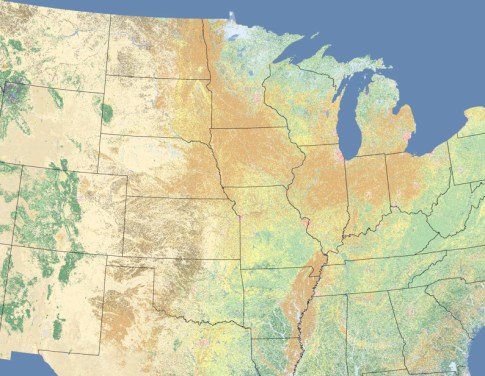
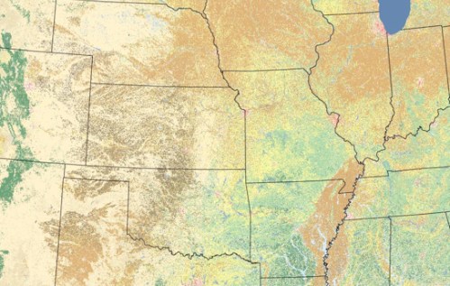
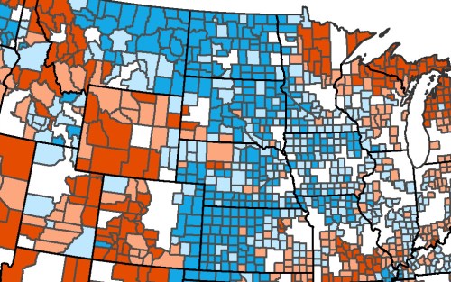
The layered images of farmlands that I consider in this post create a basis for future interactive analysis. Even without snazzy animations of time-lapse imaging of Google Earth or Google Earth Pro. By doing so, this post hopes to raise questions about how the relation and use of cropland to American agriculture might be most effectively mapped to would bring greater familiarity with the dilemmas of farming and agricultural practices. At a time when most are increasingly more unfamiliar with the organization of agricultural life that with the rising of the tides, we are all too ready to view agricultural practices in a purely macroeconomic–rather than environmental–lens. Although we imagine the agrarian landscape as an unconstrained or open space, the visualizations offer insight into what might be best be understood as a complex mosaic not only of individual interlocking ecological regions, as this ESRI visualization of the High Plains, Corn Belt, and Great Plains, but a complex economic dynamics it conceals. For despite its accuracy, and the differences between bioregions and eco regions, the unified landscape indeed conceals the divides created by the now dominant (if warped) view of each eco region as a source of crops on a global market–a view that has informed the rural landscapes over the past twenty to thirty years, from corn belt to the wheat fields to High Plains.

For as much as map nature, the division and conceptual of agricultural space in America is effectively under-written by the world market’s orientation to its products, rather than to the individual farm as a unit of farmed land. There has been something of a cognitive re-mapping of the national agrarian space, not only in terms of the needs of local bioregions or the diverse needs of bioregions that distinguish the alleged uniformity of agrarian expanse, that turns around the greater significance of cropland as a term of economic value, based on the extraction of grain or grasses from the land, distinct from the management of agriculture. The change in focus–and indeed of conceptual mapping–might allow us to look at the very same verdant terrain in Moscow, Idaho in markedly different ways, even before we’ve begun to map the variety of local crops.

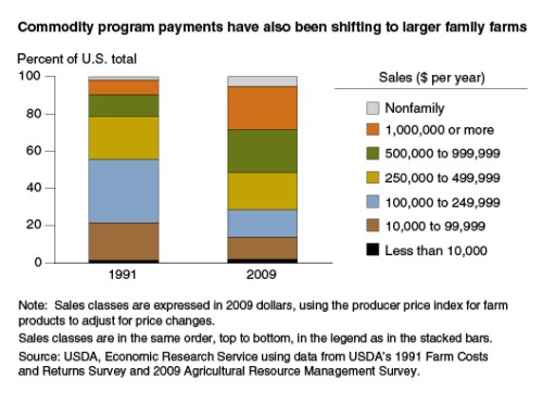
The increased extraction of goods from crop lands–from corn to ethanol to silage to switchgrass–instills a view of the commoditized landscape, more familiar from contemporary images from real estate maps of land-value than to the locally or spatially situated sense of agricultural land in a specific landscape. The shifting nature of the farm has altered the agrarian landscape in recent times: despite some debate on the future of the family farm, the deceptive average stability of the size of farms has masked the rapid expansion of small farms that has paralleled an even greater expansion of large agribusiness. The consequent conversion of most farming acreage to cropland of far larger farms has created quite new processes of food production: if the mean size of a farm is 234 acres, most cropland is on farms of over 1,000 acres, and over a third on farms of over 2,000 acres. We have seen a very recent massive increase in the sizes of farms in the corn belt and northern plains–two areas where they have more than doubled in acreage and productivity, no doubt partly in response to agricultural technologies, fertilizer, and farm-seeding, as well as to the reclamation of grasslands.

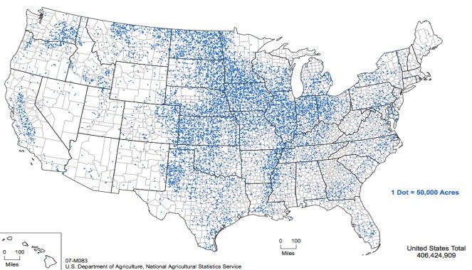
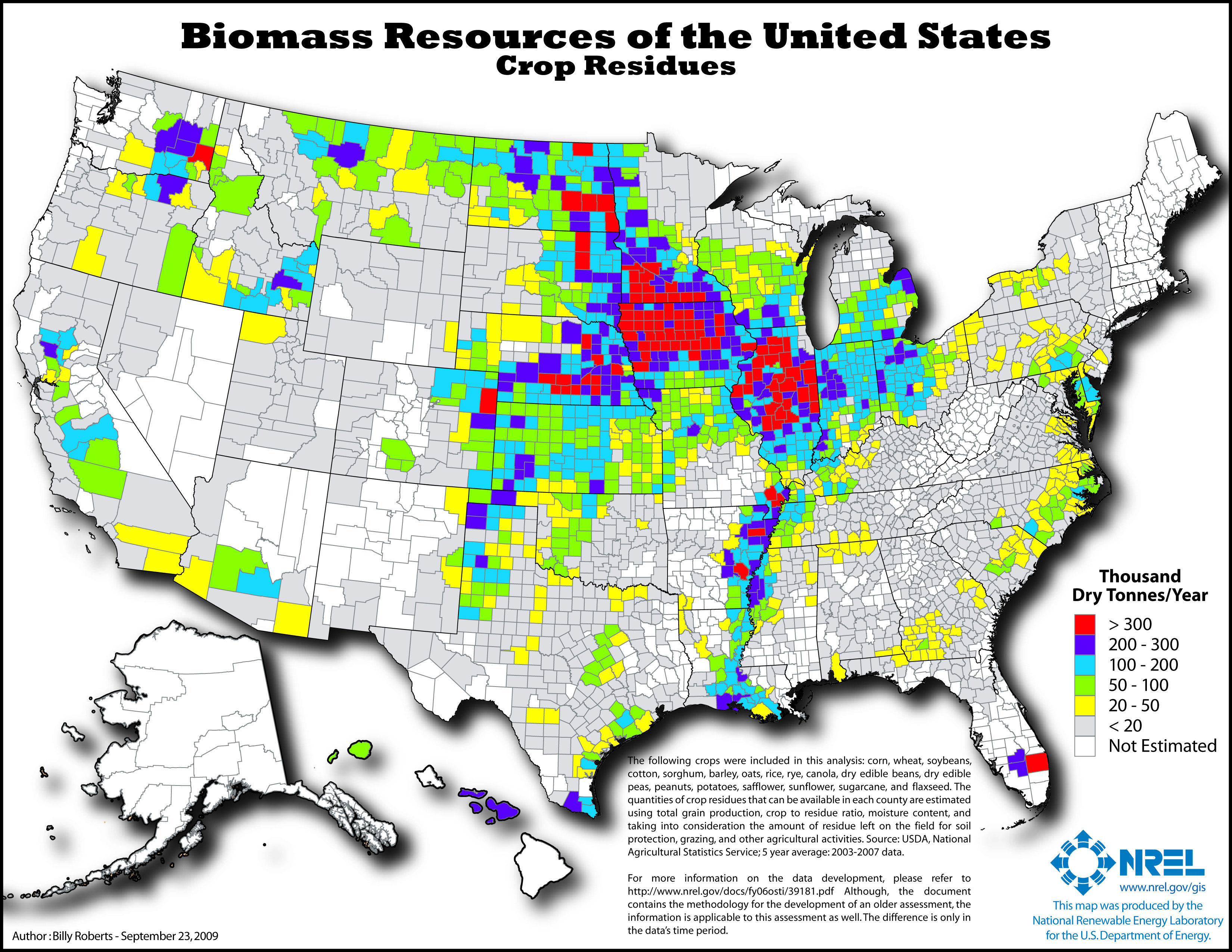
Something of a tipping point may have arrived in the expansion of farm size in these regions of the central United States, and the power of the economic investments behind them: the ecology of the landscape threatens to become replaced by the commodities we extract and map in them. By mapping the dedicated mass of biological production across regions of the country, we can se the warping of the nature of land-use that we have perpetuated in recent years, as the practice of fresh farming has become overwhelmingly concentrated in pockets of high-scale production, whereas we abandon most land to consumption in shopping malls or residential tracts, and confine a density of large-scale farming to parts of Iowa, Illinois, and North and South Dakota, and Arkansas–and one pocket eastern Florida, California and Washington.

A similar change might under-write, in multiple senses, the reframing of the agrarian landscape of the United States as a source of investment rather than view it as a single or united landscape: provocative data visualizations of farmed land in the United States suggests that we have long ago passed a similar sense of tipping point. Data visualizations are supple tools to chart notions of cropland and pasture are less rooted in place and space, and mark the results of viewing the farms in extractable units–corn or animal feed or soybeans–that shift agrarian wealth from the fertility of the lands and bounty of a region, into a map of value and investment, and often of intensive production, fertilization, and even GMO crops.

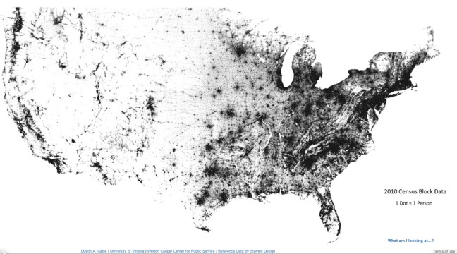
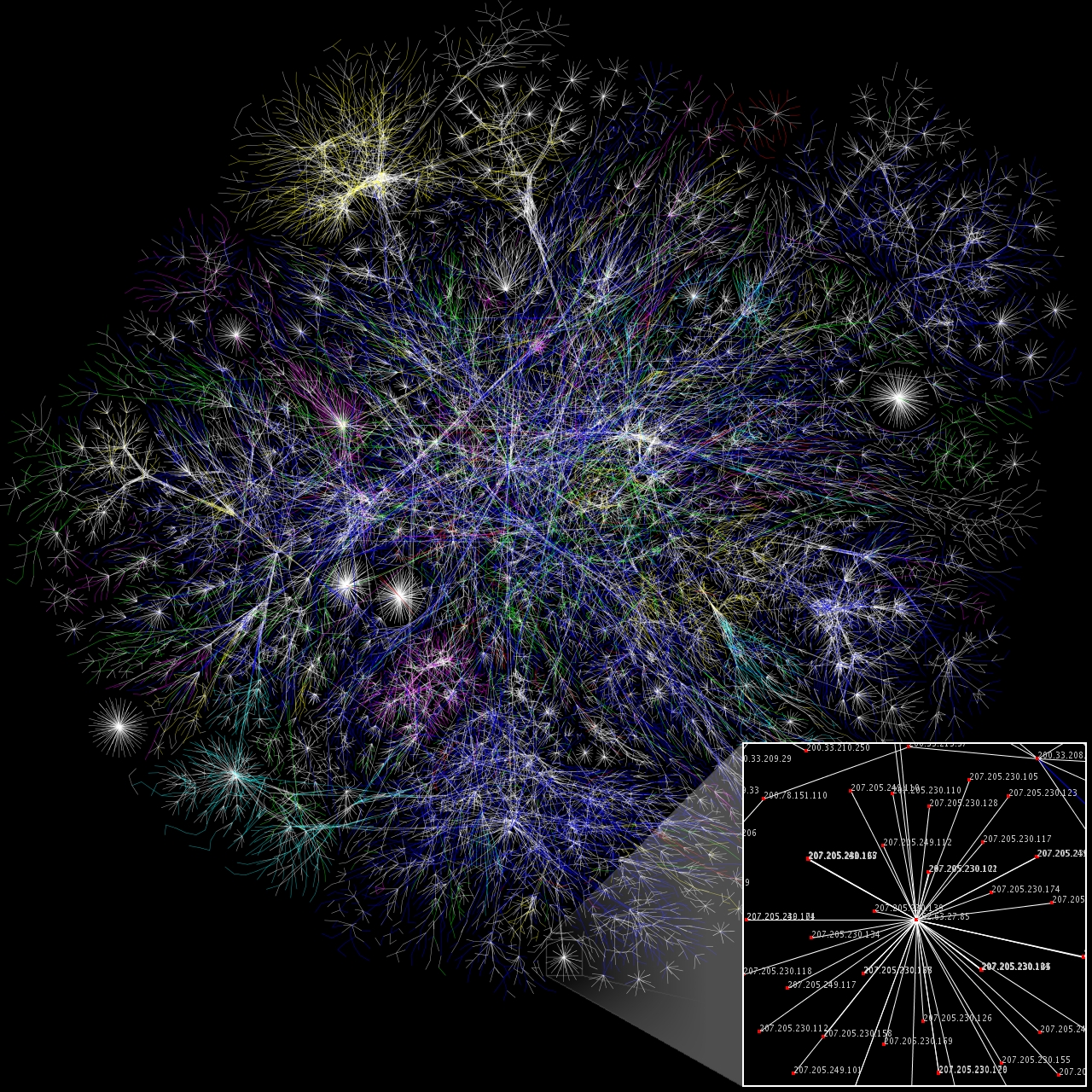
There is something paradoxical or perverse about using data visualizations as a record of landscapes, and the end is not to aestheticize data visualizations as cognitive tools–although the visualizations offer quite provocative by their colors schemes alone: the images by which the conversion and farm management of the region has created offer interesting images to meditate on both the construction and the future of crop lands, and relative coherence of the concept as a viable construction of the agrarian space with which we live and to which we are deeply attached in ways that cannot only begin to be mapped. Such visualizations of the continuous forty-eight are a useful place to begin to visualize the transformation of cropland, because their qualitative depth presents such compelling pictures of the community and of how its inhabitants use its land. Take, for example, how Dustin Cable’s mapping of Census Data by one dot per person, on Stamen design’s base-map of the nation, affords a clear division in population just west of the Mississippi River.

1. Cropland, increasingly located in the less inhabited region between the High Plains and west of the Mississippi, has been shaped by the devaluing and reframing of cropland in terms of how much can be extracted from investment. Even in the face of new stressors on agricultural land-use, from rural out-migration to the decline of the family farm to the decline of hospitable local environments, and the government under-writing of agribusiness and large farms: crops are valued have combined to create a new agricultural landscape and concomitant foodscape that was more often linked to a macroeconomic context, in place of questions of how food can get to the marketplace. The expansion of transportation has effectively removed what food we eat from where we live for most.

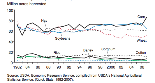
By reconsidering the range of forms of mapping farms and the use of farmlands, we must consider the landscape of farming in which we increasingly live, even if our food rarely derives from it. US farming incomes have appreciably risen since 2010-11, attracting some financial markets, but the dynamics of farming are too often based on models of extraction, rather than of nurturing the local landscape. As the production of corn has increased, since 1980, 400 percent, soybeans 1,000 percent, and wheat 100 percent, as US Secretary of Agriculture Tom Vilsack has noted, largely based on agricultural technologies and machines, including GPS seed drills, combines, and tractors, the mapping of farms have relied on being under-written by tax dollars to the tune of 30-50% by government agencies that have less regard for the mapping of farmlands. If crop insurance has helped to increase productivity some 50% since 1982, the expansion of farming technologies have shifted attention from the ecosystems and landscapes: cropland used for crops declined almost uniformly by about 50% since 1982, especially in the Northern Plains, and land-use for crops by 13%–at the same time as the amount of land dedicated to pasturage markedly increased. Corn, soy, wheat, hay, cotton, sorghum and rice traditionally constitute the bulk of farmed land; corn, soy, and wheat remain the largest cultivated crops, but the production of corn has peaked.

The range of visualizations of the changing face of farming and consequences of the emerging landscape or foodscape have neither been fully calculated or understood, and, even in an age of continuous LandSat photographs of the nation’s land cover, is challenging to map. The proliferation of maps of farmlands, from Landsat images of cropland to the expanse of regional farms, suggest a compelling illusion of coverage and expanding food production that may offer a less reliable guide to an actual landscape being devoured by agricultural machinery: if our agricultural policy is intended to bolster the strength of its remaining crops, policy has changed the landscape based on macroeconomics more than on-the-ground decisions, often ignoring place and space as construction with monocrops such as corn, soybeans, or grasses that are far from demand-based. The scarcity of water for irrigation in large part need to take stock of irrigation practices in such intensively farmed lands, in the hopes to “provide a better accounting of water use, cropland productivity, and water productivity.” The consequent proliferation of satellite-based remote sensing of farmlands provide an archive and a mirror of land use that may evoke the fear of a new form of agrarian surveillance–albeit one to encourage agreed best-practices of water conservation–but rather offer a feed-back loop to survey the recent transformation of the landscape that the reframing of national farmlands has wrought.

The striking concentration of farmed acreage in the central ten to eleven states has created a quite dramatic imbalance between the demand for agricultural subsidies and desire to control wasted water that has been so sharply contested it is difficult to agree on among elected legislative representatives. Is it possible that special interest groups might gain greater sway in the manipulation of maps to chart future agricultural policy?

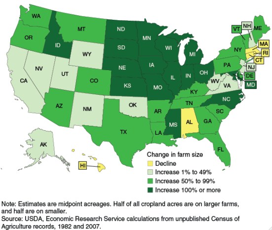
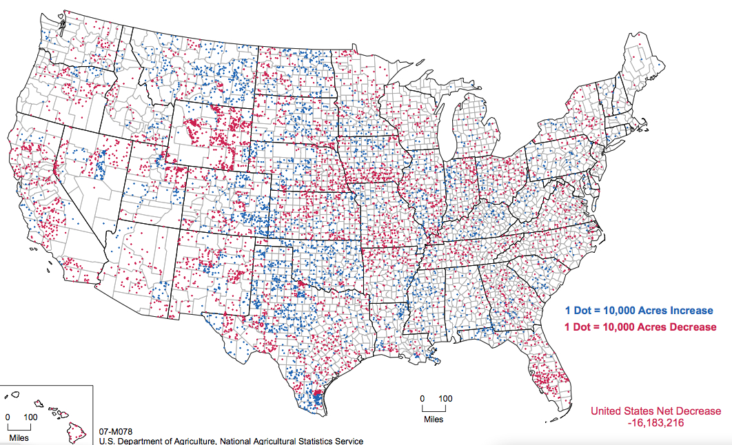
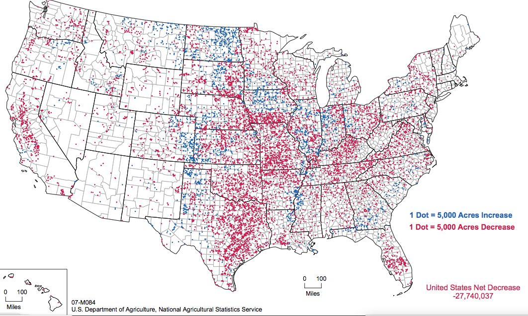
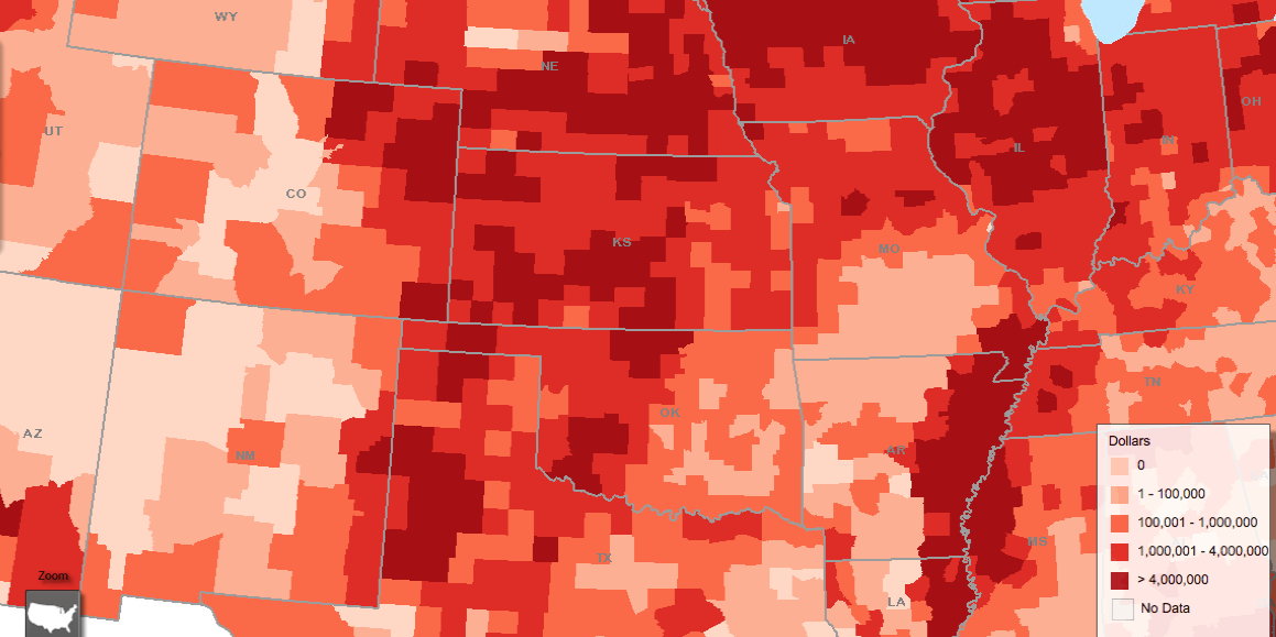
It is striking that during the period of just 2002-7, the acreage devoted to farmlands intensified in those central states, even as the nation saw a dramatic reduction in agriculture’s spread.

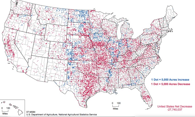
The identical period was marked by a decline in farmed cropland acreage across the entire nation that exceeded 27 million acres, a loss apparently predominantly located in the central United States, as well as California’s Central Valley and the rural South, from Louisiana to central Florida and West Virginia:

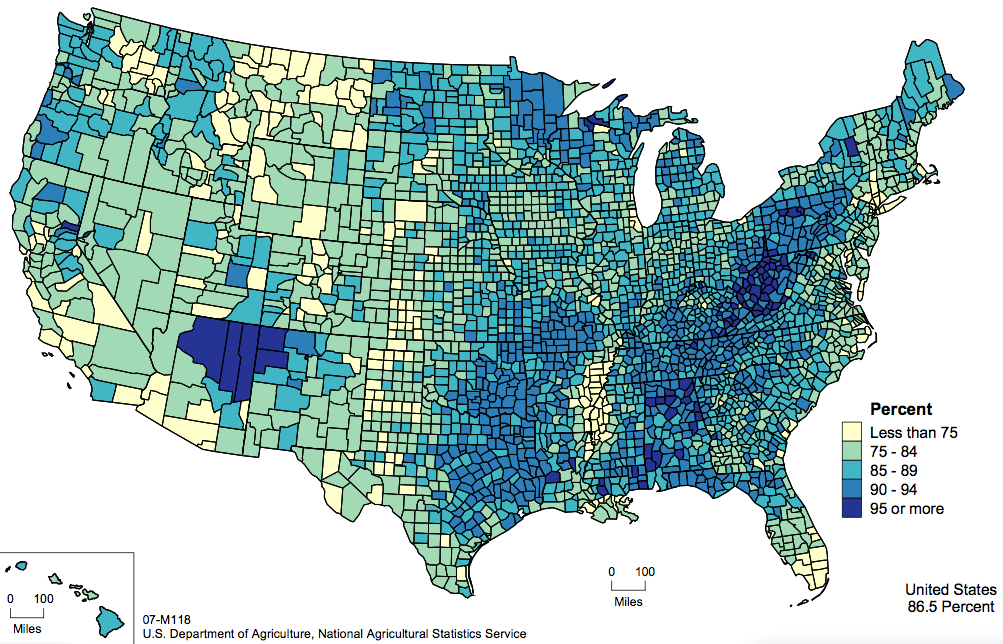
As of 2007, concentrations of those farms operated either by families or individuals were uneven in the very same regions of the central states, and in the north-central states dropped to less than 75 percent.

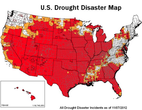
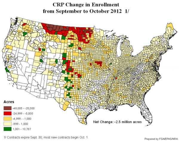
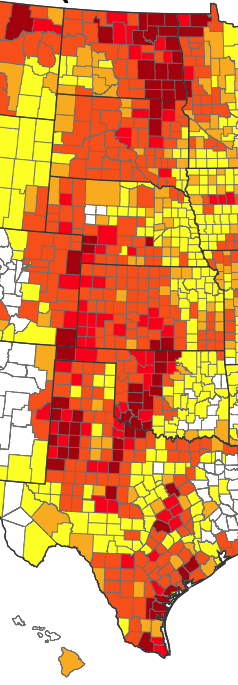
At the same time, national drought placed undue pressure on farms to maintain their profitability, as this map of the counties affected by drought through 2012, compiled by the USDA’s Farm Services Administration–and who are compelled to take up drought insurance–seems to make clear.

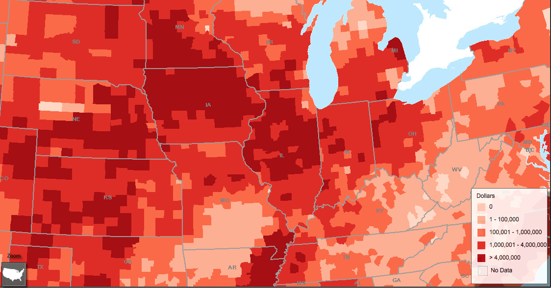
2. Maps of agricultural production reveal the increasing remove of an agricultural landscape of the nation from its cities, and from large urban areas–and indeed concentrated in a relatively restricted region of the central United States. Of the 2.3 billion acres in the United States given to agriculture, in 2007 just under one-fifth were dedicated to crops (408 million, or 18 percent)–a number that had decreased by some 34 million acres over 2002-2007. The claim to map the comprehensive changes in land-use and land-cover in the coterminous United States from 1973 to 2000–the broader goal of the professional paper–by local surveys and satellite imagery and remotely sensed data–begins to document and explain many of the deeper changes in contemporary land-cover change, to which this post returns below.

The composition of farmlands in current years suggest a marked concentration in cropland.

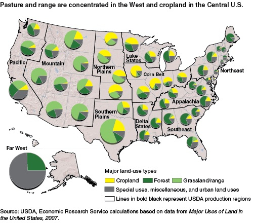
The notable concentration of cropland at a remove from urban markets (noted in grey sectors of wheels in the above data visualization) and at a remove from population concentrations defines something like a belt of government subsidies that sustain large regions of agriculture–often of monoculture crops–that are abstracted from actual patterns of habitation. It is impossible to map how this concentration of cropland came about from a disinterested point of view, but data visualizations offer a fragmented view of some of the narratives by which the landscape has been and is being shaped, and the distorted notions of place and space that they generate: the visualizations suggest a range of narratives about the effectiveness of agricultural subsidies, the foodscapes created in the rural United States, shaped through the changing relation of farming as an extraction of value from the landscape, rather than as a response to local economic needs. The shifting optic that stresses the relation of the landscape to the national economy has re-framed the landscape’s fertility.

Rather than providing a coherent “map” of the agricultural economy and government investment in farms, data visualizations offer snapshots that provide a sense of multiple narratives that shape the relation to the new rural landscape. The somewhat fragmented picture they offer present several narratives about how we’ve come to regard the farming of the land, and present questions of how to unite or reconcile the varied and discordant narratives we’ve come to tell about our tutelage of an agrarian landscape and how to best meet its needs. And they don’t add up to a collective image of a landscape that is designed to be habitable over the long term, let alone economically viable.

The problem of all these maps is how to visualize–and conceptualize–or relation to the collectivity of farmed lands that could best take account of their variety. Indeed, the possibility of mapping the mosaic of agricultural productivity must begin from remapping their relations to regional needs, in ways that are obscured by privileging their relation to commercial products and food markets, as opposed to food needs–or the value of locally produced food. The multiple mechanisms by which the state and government has chosen to invest in agriculture–and promote the production of certain products on farms, to the exclusion of others–have historically shifted away from traditionally microeconomic understandings of the farm and rural agriculture to more macroeconomic questions in ways that are difficult to map, but have rewritten one’s relation to the land and the obscured the landscapes that they have begun to change.

3. The remote-sensing of shifting maps of land cover in the United States is extremely of the moment, and not only for the impact of climate change. It may be odd to present data visualizations as a landscape, but as indices of both productivity and indebtedness, regional map-based visualizations offer ways of thinking about how the land is seen in ways that have not yet been fully understood. For if the mapping of rural America and its agricultural productivity are increasingly contested, the landscape . Maps of farm subsidies offer telling mirrors of the extent of government investment in agrarian expanse. They provide a sense of the expectations for the value of land-use, and frame the image of productivity one would want to produce: but they are also the result or end-product of the negotiation of local demands, by tracing an image of the changing face of farmed land riven with debts, subsidies, relative lack of profitability and indemnities, the bulk of which go to larger farms, that expand to make up for the sizable decline in farmed acres.

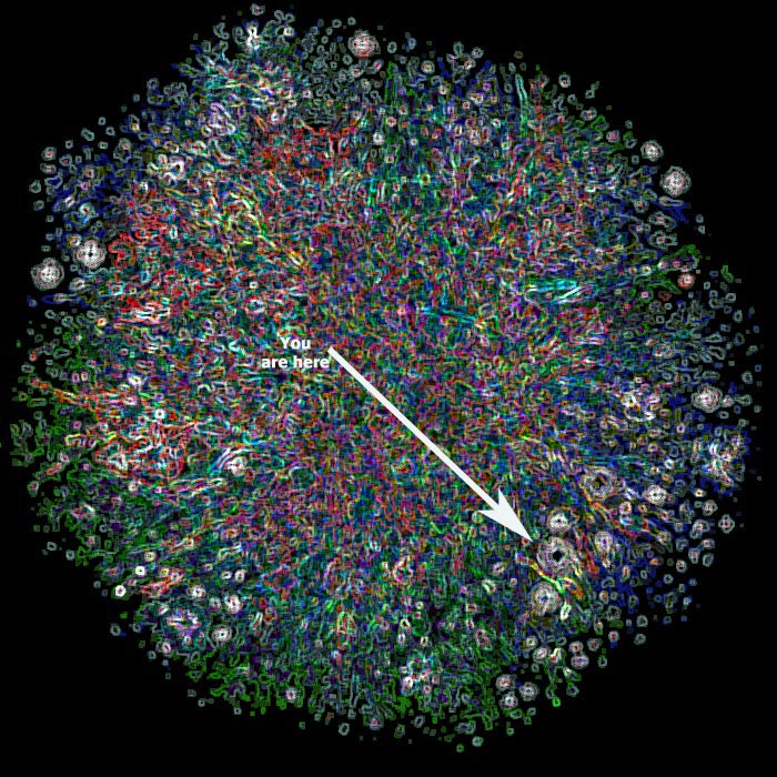
When we map the huge levels of out-migration that occurred from 1980 to 2000–or from the Clinton years to the Bush years–marked by a decline of the population of the so-called “corn belt” in Nebraska, Iowa, southern Michigan, and Kansas–we can see the changed character of the rural landscape in America, as much as by the huge decline in crop diversity about which I’ve blogged in relation to the expansion of agricultural production that has been fed by agricultural subsidies–monocrops that maps of food reveal as having far less reference to a region or place, at a remove from urban areas of consumption that do not best serve populations. The shifts in settlement away from the central US were clear long before 2010, but the distribution devised by Dustin Cable maps from that year’s Census maps a starkly blank central and west, into which extend feathery wisps, clinging to roads and interstates, the new rivers of rural settlement.

The long-term but recently drastic population declines from the Great Plains and Corn Belt have been a prominent back story on the remapping of American agricultural diversity, as has the declining revenues and work associated with farmlands, often worked by fewer and growing crops with greater intensity; losses of population in rural regions orient the viewer to the shifting national foodscape, whose image of dwindling population in non-metro areas reveal stressors on the economic structures of rural agriculture, and of the relation between urban and rural lands, or between the expansion of farming to meet the population growth of urban areas. (This population shift that can also be charted by the expansion of “Heat islands” of “impervious surface area,” paved urban and extra-urban areas, mapped by Landsat images and night-time lighting, that exert disproportionate influence on climate change and remove a sense of urban settlement from agricultural space.) The loss of populations to some extent mirror the decline of family farms and rise of agribusiness, which tries to meet growing population needs.

This picture gains another layer of complexity once we consider the infusion of government subsidies to agriculture in the very same states–subsidies inflating monocrop cultivation that have created a new map of the country’s farmlands, over the decade dominated by the previous Farm Bill, and created a new and unprecedented level of indemnity and indebtedness in farms that are now considered as cropland, but often face too little water to be productive. While funds were distributed, they were concentrated in the same area where economic profits declined, and family farms shuttered–and an overall decrease in cropland nationwide was offset by increasing amounts of land dedicated to pasture and grasslands, according to the 2011 USDA ERS report. There is a tortured logic of dedicating increased land to corn and silage as animal feed: since it takes 10 to 14 pounds of grain-based feed for a cow to gain 1 pound of flesh; subsidizing animal feed is an outrageously uneconomic way to produce our food supply–although the international market for American meat is high.

Many of the same farms and acreage of farmlands are enrolled in federal crop insurance, changing the complexion of farms and character of government subsidies for land and increasing fear of their indemnities–and an increasing amount of farms enrolled in insurance programs nationwide, but especially dense in areas where state farming programs are established.

4. What are the reasons for this investment, aside from the desire to keep the local economy afloat in hard times? Despite the relatively restricted regions of intensive planting of subsidized crops, we remain tied to the mindset of a picture of the nation’s economically productive landscape as it was imagined circa 1940, when one-third of the world’s production of corn came from the central states, and half of the farmers in the central United States were tenant farmers:

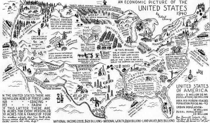
The current agrarian landscape has sharply diverged from one where 62% of global production of oil was located, 52% of the entire world’s corn was harvested and Grade “A” farmland existed across the Midwest. But the attempt to invest money in the landscape to bolster its production of economically desirable products that might perpetuate this image, even at the expense of local farms and rising levels of indemnity. Protectionist legislators have continued to write into and perpetuate in our most recent national Farm Bill, although that landscape no longer exists, even if it struggles to support the image of a fertile range of grazing and farm land in the “Nation’s Bread Basket” in a land where subsidies are crucial and indemnities endemic, and local ecologies often overlooked.

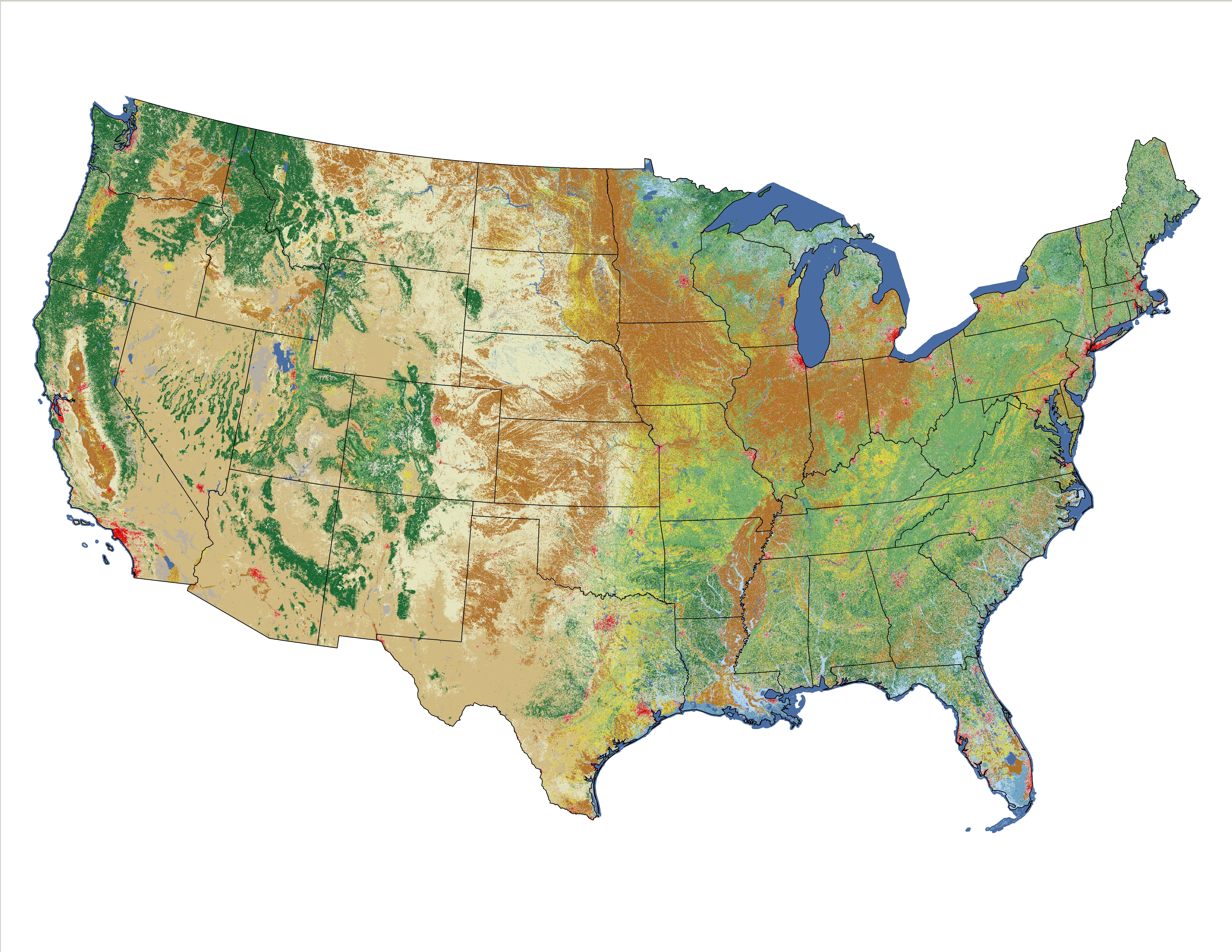
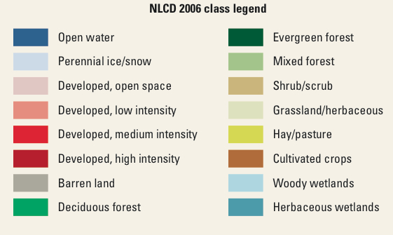
The more restricted areas of cropland, combined with the recent expansion of federal subsidies to certain areas, regions, and crops reflect the relative constraints of crops within the national land cover–whose row crops are measured below across the coterminous United States–can be traced from 1992 to 2006, with special attention to relations of row crops (light brown), pasturage (yellow) and shrub lands (tan) in the central states–noting the tortured logic of dedicating cropland to animal feed if it takes 10 to 14 pounds of grain-based feed for a cow to produce but 1 pound of animal flesh.

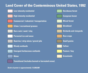
The Multi-Resolution Land Characteristics Consortium from 2001 reveals deep inroads of grasslands–with a slightly changed color-scheme–at a stunning spatial resolution of thirty meters, using remotely sensed Landsat Enhanced Thematic Mapper+, to differentiate land cover, and show an expanding northwest and midwest, even if the changes are slightly exaggerated by a stronger color spectrum–in which it almost seems that the physical remove of these row-crops from agrarian needs creates its own internal economy of production that has altered how cropland is conceived across the central states.

USGS Land Cover Institute (LCI), 2001

The 2006 wall-to-wall land cover database, although it groups crops collectively, shows increasing inroads of pasture (yellow) and grasslands (lightest green) and slightly diminished cropland:

It might be compared to the highlighting of pasturage in a lighter almost neon green in this USDA map of cropland layers of 2009:

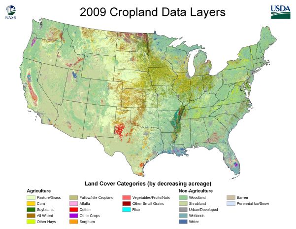
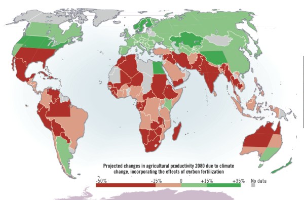
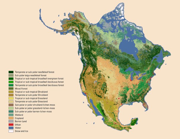
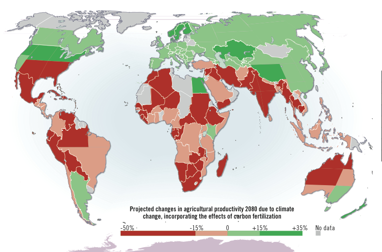
5. The increased incursion of grasslands, pasture, and silage into the cropland in the cover layer conceals the deeper changes in the organization of agricultural expanse–but also masks the sort of crops that are growing in each region–including the expansion of corn and soy. Given the complexity of processing these groundcover maps, a sequence of data visualizations might reveal as a radically changed landscape both of government intervention and of expanding monocrops. As a point of contrast, however, the North American Land Change Monitoring System monitored the land cover of all North America in 2005, using Moderate Resolution Imaging Spectroradiometer (MODIS) to reveal the far greater expansion of cropland to the north–an area projected for greater future productivity of crops such as wheat, due both due to lower rising temperatures and the expansion of arable land for growing wheat, canola, and barley in all Canada by 15% in a 2008 United Nations’ Environmental Program map based on predicted “increased temperatures, precipitation differences and . . . carbon
fertilization for plants,” while American productivity of crops is predicted to drop some 15%-50% on account of the impact of climate change.

The image of arable land above the 48th parallel indeed seems much more expansive, anyways, and even far more fertile with crops today–not only due to a different structure of state subsidies, but also to different agrarian practices, and a high-speed rail dedicated to transporting grain to across the country.

The relatively restricted cropland in the United States was balanced by, oddly, an expansion of land dedicated to agribusiness crops that were less dedicated or directed to the dining table, and to an increasing mountain of investment in ostensible farmlands.

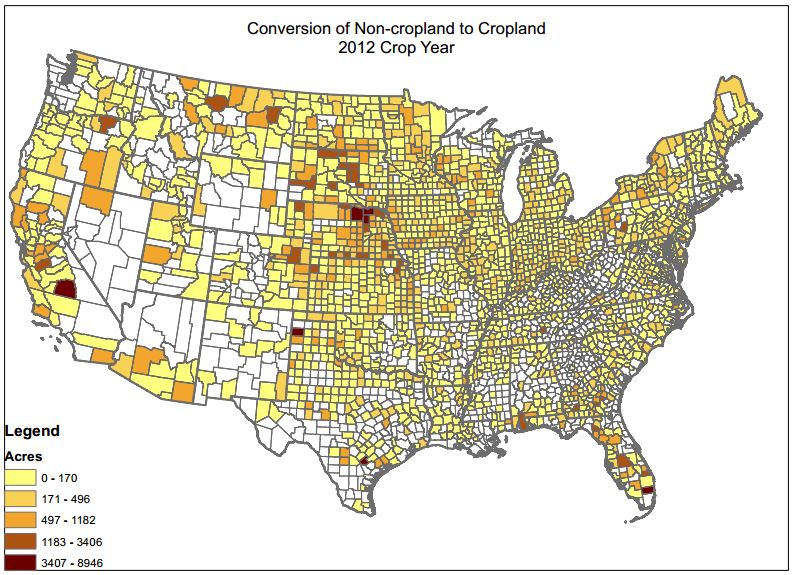
There is some evidence for the bad effects of the unmitigated expansion of row-crops in the landscape of the central United States. For the area of American cropland include a conversion of a substantial amount of land–2.5 million acres–from the Conservation Retention Program to the growing of soybeans and corn in North Dakota and Montana, creating some total plantings of some 97 million acres on formerly CRP lands since 2007, largely to the benefit of large agribusinesses who employ monoculture plantings, with a huge impact on the local landscapes.

The distribution across the country partly reflected a new “map” of how agriculture gained USDA appropriations to expand the growth of crops that might not necessarily meet food demand. Although the investment in agriculture lumps subsidies, disaster relief, crop insurance premiums, and conservation programs in an area effectively costs the nation; questions of such spending are perhaps too significant to be determined by guidelines of a single Farm Bill. In this map, farms have increasingly met needs for feed, fuel, and fiber, even while using less cropland to do so–and the design for subsidization was warped through the different agribusiness and corporate interest groups that may well have led legislators to concentrate resources in specific legislative districts, with limited investigations of their long-term effectiveness. Despite a massive conversion of nearly 400,000 acres of grasslands into cropland in 2012 alone, such “sod-saving” provisions in the Farm Bill are difficult to secure; states so notorious in converting grasslands to agricultural interests–like Florida, Nebraska, or South Dakota, and Iowa–to be known as “Sodbusters” seem indebted to the promise of jobs that big ag might secure.

A similar logic seems to play out in the receiving of agricultural subsidies to encourage the development of farmlands, most often with an eye to farm futures rather than local needs.

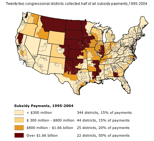
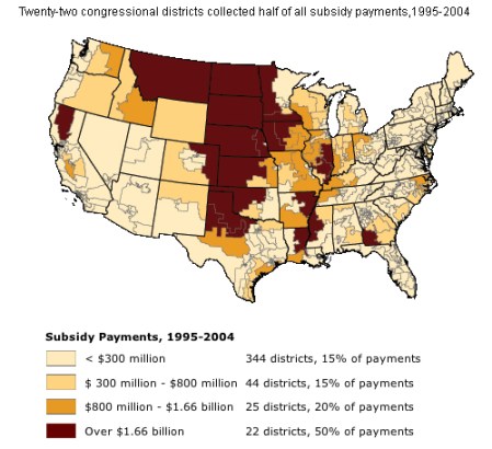
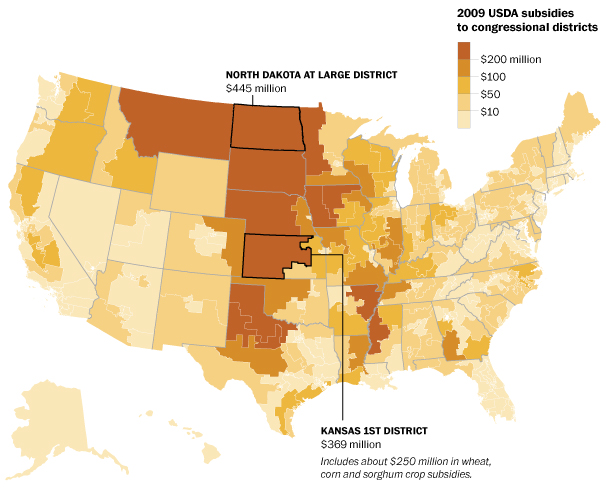
As a result, states are not directly subsidized–or farmers, for that matter–but the Department of Agriculture allocates funds to districts, creating a new map of the economy, as much as a map responding to needs of crop-cultivation or food-needs, based on this map of subsidies collected in bulk by some twenty-two congressional districts in the decade 1995-2004.

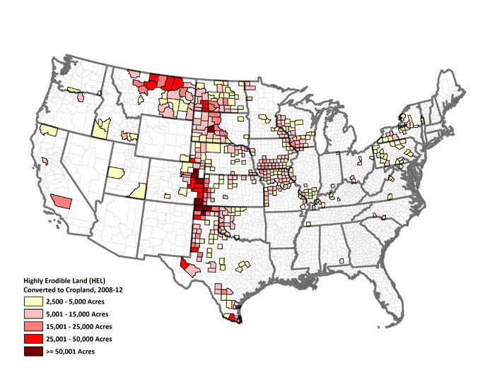
6. Such representations reflect the realities of the shifting agrarian landscape. They offer resources to refine our picture of the land by delineating varied concentrations of national resources by government investment. These representations of agrarian landscapes serve as a gauge to negotiate our relations to reality, as much as to measure them, placing into visual relief how we project value onto agricultural landscapes without attending to the specificity of their character–and tend to link value to the continued economic productivity of rural lands in ways that deny local changes. This even extended to the conversion of much “highly erodible land” (HEL) into cropland for moneys from 2008-12, often to intensify the farming of subsidized corn and wheat, filling areas from Montana to Texas that are centered in what was once a Dust Bowl devastated by persistent drought.

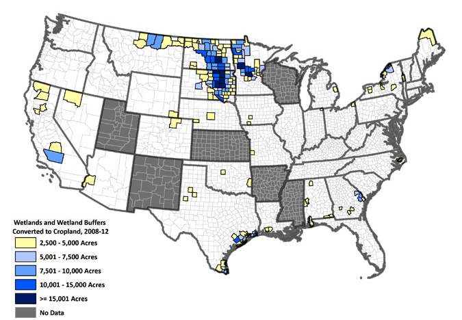
This occurred even as large numbers of wetlands, also important wildlife habitats of their own, and wetland buffers, were were also being converted to cropland in many of the same regions of the Dakota prairies, Montana and Minnesota, adding up to a loss of far over 15, 300 acres each year from 2001 to 2011–most (60%) in order to plant corn and soybeans.

The individual county costs for such conversion of such acts of bad agricultural stewardship averaged, in the case of counties loosing wetlands, $10.1 million, and in counties of highly erodible lands $5.8 million–four and two and a half times the national average respectively. And particularly notable seems the expansion of conversions of either both wetlands and highly erosive lands (framed in violet), or either wetlands (framed in sky blue) or erosive lands (framed in light green) both in Montana, upstate and western New York state, Texas and in northern California, suggesting a diffusion of bad practices of land-reclamation at much cost.

7. How much does this actually cost the government? And is this level of investment and subsidization financially sustainable? If one filters data and divides subsidies per inhabitant of rural regions, the largest six programs of USDA funds pump debt to diminished rural populations at astounding rates; if farming remains less profitable, it has gained and retained legislators’ ears for continued support for subsidizing crops as corn in areas of low population–dominated by agribusiness.

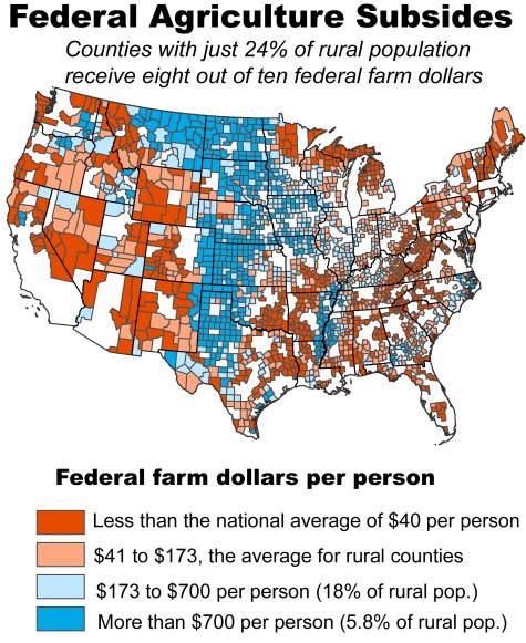
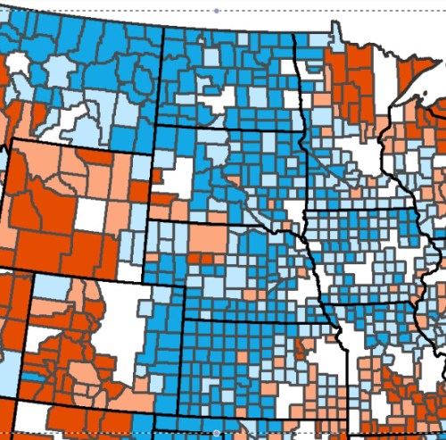
Despite the typo, the map displays an astounding concentration of relative farm dollars in North Dakota, South Dakota, and Nebraska–as Kansas, the southernmost state shown in the below map of subsidized farms in local counties, and bright blue Montana in the upper left.

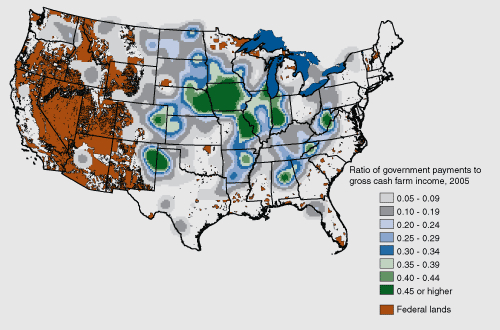
The limited profitability in many of the very same regions–and indeed the focus of profitability only in states of the corn belt such as Iowa–suggest the deep economic constraints about such macroeconomic policies, and the limited success of farm income in many of the same regions in 2005–even as governments have shifted their investments to larger farms–with under 30 percent of farms receiving commodity program payments in a typical years. Indeed, the shift in the allocation of funds to farms with higher incomes and higher-income households has encouraged commodity-related programs–like grain sorghum, wheat, oats, or soybeans–that are removed from real food needs, and creates a picture of radical imbalance for the smaller farm, privileging “high value crops” in a macroeconomic sense, in ways that were often removed from actual farm income in many regions outside of Iowa, Nebraska and select parts of Missouri and Texas in this map of 2005.

The shift to larger farms whose incomes actually far exceed average household income in recent decades created a new dynamic of regional and rural investment that has privileged a food trade removed from local needs or a variety of foods, and considerably increased the percentage of non-family farms in ways that seem poised to increase over future decades.

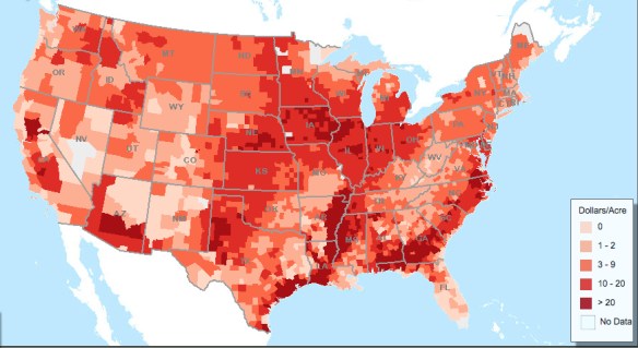
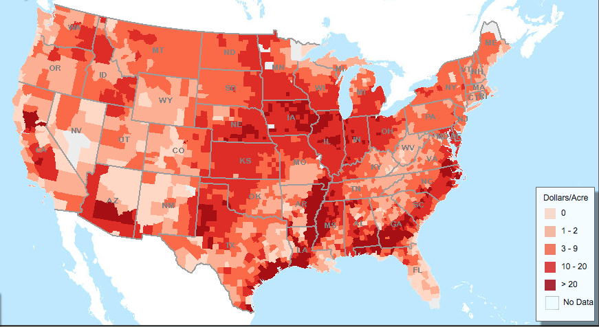
Are the results even profitable? The level of indemnity is striking. There is not only considerable variation in crop indemnity nationwide, but evident intensity in regions of greatest population loss that are relatively removed from metro centers:

The patchwork strip of heavy indemnities of over $10 million per county, designated in dark brown, that run across the center of the country in 2010 (and are particularly concentrated in North Dakota, Nebraska, Colorado, Kansas, Oklahoma, and Texas–all big foci of federal farm expenditures) raises question of the allocation of farm dollars in any Farm Bill, and indeed how to encourage local best practices with federal policies. Can such levels of indemnity be fiscally justified as a food policy?

How do they indeed distort the sort of food policy that the government might want to encourage? The question of best managing the balances of investment in the continued productivity of farmlands may have been too long framed in macroeconomic terms removed from local markets or best food practices–farm dollars being dedicated to the production of grains not destined to be consumed by human mouths, and whose cultivation imposes increasing costs for limited exchange value. Are these losses concealed in most maps of investment, and what sort of image of crop production do they effectively produce?

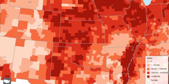
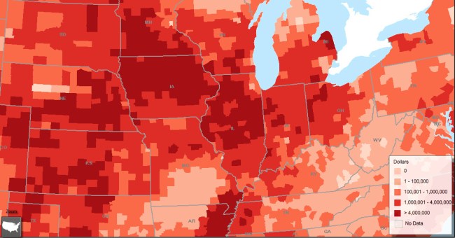
Some of the same states are highlighted in the below, more detailed, map of such direct and counter-cyclical payments–those payments that depend on weather changes or currency fluctuations, rather than cycles of agriculture–emerge in the recent he Farm Program Atlas, mapped for the USDA by Anne Effland, Vince Breneman, David Nulph, and Erik O’Donoghue, mapping variations in the dollars received by local farms in 2009. (The atlas will be completed through 2012, but this map provides an initial snapshot of where the money goes, county by county.) It offers a baseline of a picture of the benefits that the seven largest USDA programs give the nation’s farmers that is likely to be a touchstone in future debates.

The fluctuations charted respond to global markets and profits on crops, now removed from the calculus of local, regional, or national needs. Given that in 2009 corn and soybean prices were extraordinarily high–too high to trigger counter-cyclical payments as well as the direct–they offer an image of direct crop payments. And the image of direct cropland payments per acre is not in fact drastically different or distinct in its complexion, if it lightens the amount expended in the Northwest, Kansas, and Nebraska:

(If one were to look only at the counter-cyclical payments for that year, however, the rise in prices would make most monies appear devoted to the South for that specific year:

The different image that this provides of dollars spent in the Southland, however, is effectively a distorting mirror of the continued monies that flow to the acreage in the corn belt and across the midwest.)

If one charts the picture of the proportions of base acreage receiving either direct or counter-cyclical investment in farm dollars, a similar clustering of density emerges specific to the Midwest that suggests the remove of crops either from centers of population–metros–or areas of dense population–and even something of a marked inverse relation to population density:

The below map breaks down variations among individual counties that received dollars in ways that offer something of a mosaic not only of government investment, but a map of the competing interests that defined the future of our land use in states as of great population loss–and increased allocation of dollars/person–like Nebraska, Iowa, and Kansas, suggesting considerable local variations perhaps based on local agitation.

What this means is not only an increased investment in large agribusiness, but a skewing of investments to areas removed from urban populations in the mosaic of those areas where federal farm dollars are received, and over $700/person of farm subsidies arrive yearly.

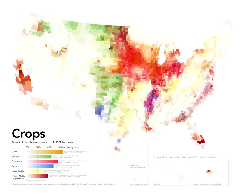
It is the underside, as it were, of increasing “over-specialization” in agricultural production and in the agrarian landscape–and the divorce of that landscape from our changing national foodscape, whose disproportional warping over the years has been described and charted by William Rankin with visual eloquence, revealing in five colors the recent expansion of monocrops in corn (orange), wheat (green) and soybeans (red), destined for agrarian feed at considerable expense both as an investment and a use of land. Local economies, such as they exist, are sustained by agribusiness–the largest property owners in many of these states, who privilege a uniformity of crop.

8. The most dangerous implication of this mis-managed mapping of federal investment may lie in the removal of local needs from a sense of what crops are being encouraged or discouraged by the USDA, creating distorted foodscapes evident in how the below map of William Rankin clearly reveals the disproportionate amount of farm dollars dedicated to specific crops–and to practices of monoculture–that are most often removed not only from the food needs of urban areas or urban poor, but run against both good agricultural practices of local variation and environmental health.

And just to focus on the monolithic intensity of Soybean and Silage in one area, one can see how little of the per capita funds spent by the USDA on agricultural acreage actually reaches the tables of Americans, or might contribute to their dietary health.

US Government data, relatively recently released, provides a shockingly similar distribution of funds picture of roughly the same area received in subsidies, as of July 11, 2012:

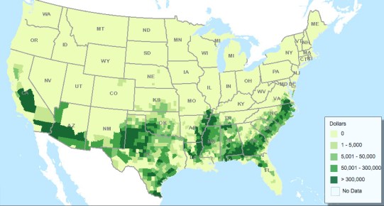
9. The dramatically lopsided geographical distribution that results among farmers’ markets across the nation–those ever-present upbeat small-scale micro-economies of the food trade–is no surprise: even when providing the select with “fresher” food, such markets are removed from very centers where those subsidies arrive–the inaccessibility of those markets in the major metros to folks on SNAP programs (or food stamps that the farm bill guarantees) is no surprise because it is a sort of niche agriculture in an age of the homogenization of crops, and the withdrawal of industrial agriculture from produce:

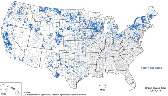
For organic farms largely spread to areas located outside the most intensively farmed acreage in the US by 2007.

Where have the organic farms gone? Outside of the corn belt, in part, although the clearly cluster in many areas of Wisconsin, Minnesota, Montana and Iowa, but often in the Northeast, Northwest, and Central Valley of California, the great producer of nuts, fruits, and vegetables.

What happens to larger markets of food when areas of the concentration of fruits such California’s Central Valley face sudden drought? Just stay tuned. It’s most likely coming to a food-stand near you.the USDA’s Economic Research Service, using data from the Agricultural Research Management Survey

1 Comment

Filed under data visualization, ESRI, foodscapes, USDA

Tagged as agribusiness, agricultural subsidies, croplands, Farm Bill, farm size, farm subsidy, farmers' markets, farming subsidies, farms, food policy, monocrops, Tom Vilsack, Whole Foods, William Rankin

February 1, 2014 · 1:26 pm

Internet Maps for Geeks Only?

Navigating the sea of information that encompasses most of our worlds and flows around our lives creates such steep challenges of spatial awareness that we are often not easily oriented to: and the increased overlap between the sea of information with the sea of our economy–so that the two sometimes seem to be congruent with one another–suggest that they have become an ecoysystem of their own, with its own eddies, shoals, currents, deep water inhabitants, predators and low-lying, and scavengers: it contains multiple life-cycles of interdependence, as well as multitudes, and whose data flows create their own habitat for those who dwell in them, and move “Alive in the[ir] Sea of Information.”

If we’ve only started to map these new ecosystems, their transposition to a rehabilitated fictional cartography offers a start.

The routes of travel and communication that are woven on-line on the world wide web challenge the limits of human comprehension of space or of an inter-related network: links created by on-line communication provide compelling bases for surveilling individual locations by harvesting metadata in hopes to establish and track an individual’s physical position through a vast database, employing a physical network cell phone towers as tools of triangulation to track the real whereabouts of their users. But on-line traffic constitutes a web of big data that remains impossible to comprehend in its totality–and that none of us have the mental tools to process; the multiplicity of links, channels and interconnections it presents challenge clear formats of spatialization, in ways perhaps comparable to how the emergence of “non-places” from airports to hospitals to internet cafés, challenge the definition of an inherited notion of “place.”

Can one imagine the map presenting us with an indicating arrow, “You Are Here”?

The lack of orientation it offers makes it perversely comic.

This is, perhaps, why it is pleasantly reassuring to see the ultra-detailed old-school “Map of the Internet,” compiled so painstakingly after a Rand McNally five-color atlas by the amateur Slovakian cartographer and graphic designer Martin Vargic. Consciously modeled by Vargic to echo the familiar patient didacticism of the maps long included in National Geographic, whose conventions and symbolism have been so aptly interpreted by Denis Wood and John Fels, the “Map of the Internet 1.0” came out from xkcd this fall of the internet with limited fanfare; Vargic takes the notion of a “data-stream” to its geographic analogue of aquatic spaces, where Data Streams feed Data Oceans, Information Oceans, and Spam Oceans that swirl around inhabited or colonized continents of servers, replete with a comprehensive detail that perhaps predominantly appeals to geeks alone, were it not for the comically retro reserve of its staid 2-D conventions, overloaded with densely positioned text in the manner of a National Geographic map.

With a toponymic density so perfected in the medium of the old National Geographic paper fold-out maps that it is hard to read or replicate on the small screen, the map is both a romantic look back at the conventions of mapping the boundaries of sovereign territories in a globalized world and a projection of a world that has come to colonize our minds. (If it might truly be suitable for classroom use–if for what sort of kids it’s hard to imagine.) But the map is also for us: for much in the way that early world maps engraved and designed by the cartographer Abraham Ortelius offered their readers meditative ends in the sixteenth century, bedecked with stoic maxims, we can gain some stoic remove from the web in this culturally reassuring map, the density of whose textual content calls for the sort of close-reading close to the pure pleasure of map-reading.

As we explore this map, we exult in its copious detail, encoded, to be sure, in the format of a geographic map, but coming perilously close to a childhood pleasure of a land of imagined travel. Exploring the detail of multiple fonts that alternates boldface, italics, and capital letters, we can navigate the near proximity of Database Ocean to the shoals of the Sea of Copyright, crossing the land of Flickr to the Sea of Archives where we find our Mega Uploads, viewing the oceanic currents that might carry our craft to different regions, or veer off from the Sea of Copyright to the smaller, protected gulf of the App Sea monitored by the App Store on Apple.

Or, if we’re not so versed in currents of code, or the unpredictable currents of the Circumpolar Datastream, doing our best to avoid the perils of the Zuckerberg Gulf or the remote island of Second Life, we can find ourselves in familiar territories below the Interface Sea, or in the lands of LinkedIn, Facebook, Twitter, Yahoo, Pinterest, and Reddit, remotely adjacent to Wikia, on the one hand, and, on the other, the Sea of Art–and World of Warcraft–which we might be far more ready and prepared to navigate and explore, without descending south to Google.

Off of the Ocean of Information lies an opportunity of repose for the buffeted traveller, below the looming megastate of Microsoft, and beside the Programmer Ocean, safely out of reach of the domain of Spam, nourished by the warmer Datastream of Ideas that washes its coasts, where iTunes is established and Android can be accommodated, and even Blackberry constitutes an offshore isle. In this land, Innovation Sea is a fertile breeding ground of speciation, itself nourished by the whirls of the Datastream of Ideas.

Vargic maps a particularly entrapping set of perilous eddies of ocean currents around the more shady criminal elements of the web and the land of porn it has spawned, duly noted on the map as a newly discovered body of land–an illicit region bordering on internet crime and piracy, which would of course be magnified if he chose to map not the framework of the internet but actual web-traffic or internet use:

The loving rendering of the internet as a patiently designed map of a world we are probably too familiar inhabitants comically lavishes graphic attention on virtual media of communication which pride themselves on being paperless: the map employs or revives a familiar artifice of mapping as if to render transparent the dramatic expansion and proliferation of a diversity of radically disembodied forms of reading online by highly conventional signs and forms of design, as if we could readily see the webs of information, servers, platforms, and providers that might more aptly be figured as a sea. The familiar poetics of cartographical space Vargic so ably encoded seems meant to offer, of course, an opportunity for repose as this is a recognizably domesticated terrain, as much as a terrifying Digital Ocean, whose eddies of Outdated Datastreams buffet the traveler, and where Encoded Torrents terrify the mariner who ventures to far offshore. There is the scary less-known regions that correspond to the poles, and echo early modern maps in their reference to terra incognita (Hic Sunt Dracones–a legend that rarely appears on an actual map, and never appeared in the medieval maps), below the Digital Ocean–if not exactly remote, the Great Southern Land is the somewhat terrifying terrain of Floppy Disk Plain and Steve Jobs land. (The But the copious abundance of written meaning that lies across the map offers a return to the pleasures of map-reading in an age of Google Earth.

The not-so-subtle beauty of Vargic’s map is that it uses familiar conventions as a way to distance ourselves from the world of data overflow, the information overflows of the Ocean at its center, whose azure waters lap the land of Google but maintain their autonomy from it, at the same time. And those huge internet companies–Cisco, HP, Oracle, IBM, Microsoft–are comfortable or credible regions on the map, where we might just decide not to go. It’s not only for internet geeks, but is something of a stable refuge, on a virtual piece of paper, from the heterotopia of the portal.

	Evergreen on Weed Maps?
	Evergreen on Weed Maps?
	Dave on Maps and Metaphors: Boundaries…
	Daniel Brownstein on Eternal Borders and the Territ…
	Paul DUGUID on Eternal Borders and the Territ…
	Frances Smith Starn on Sea Surface Temperatures

	Evergreen on Weed Maps?
	Evergreen on Weed Maps?
	Dave on Maps and Metaphors: Boundaries…
	Daniel Brownstein on Eternal Borders and the Territ…
	Paul DUGUID on Eternal Borders and the Territ…

Monthly Archives: February 2014

Local Landscapes in OSM: the Shifting Economy of Mapping Place

Follow the Money from the Bay Area’s Shores

Maps for Reframing an Over-Farmed Landscape

Internet Maps for Geeks Only?

Follow Musings on Maps

Recent Musings

Support Musings on Maps!

Recent Comments

Tags

Blogs I Follow

Recent Comments

Archives

Monthly Archives: February 2014

Local Landscapes in OSM: the Shifting Economy of Mapping Place

Follow the Money from the Bay Area’s Shores

Maps for Reframing an Over-Farmed Landscape

Internet Maps for Geeks Only?

Follow Musings on Maps

Recent Musings

Support Musings on Maps!

Categories